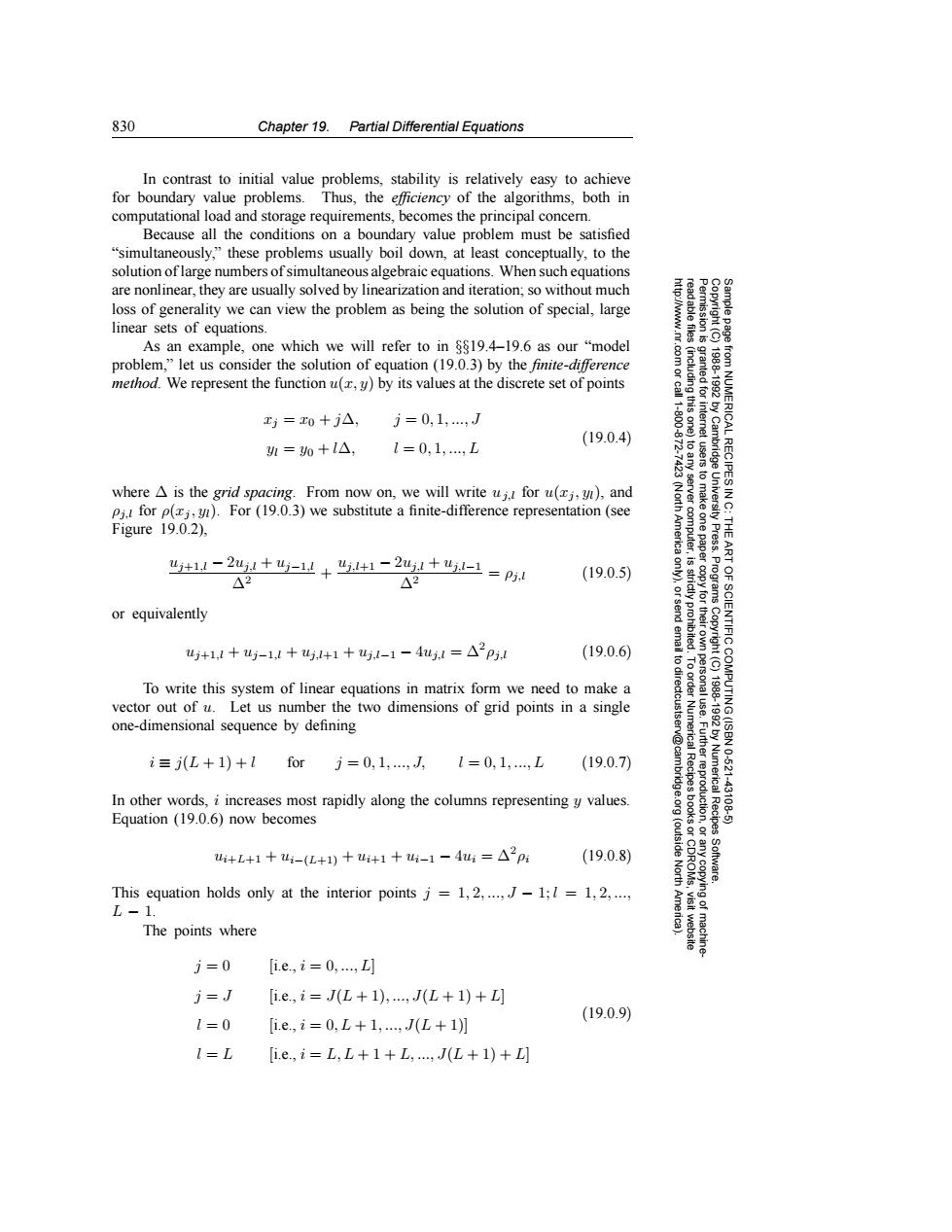
830 Chapter 19.Partial Differential Equations In contrast to initial value problems,stability is relatively easy to achieve for boundary value problems.Thus,the efficiency of the algorithms,both in computational load and storage requirements,becomes the principal concern. Because all the conditions on a boundary value problem must be satisfied "simultaneously,"these problems usually boil down,at least conceptually,to the solution of large numbers of simultaneous algebraic equations.When such equations are nonlinear,they are usually solved by linearization and iteration;so without much loss of generality we can view the problem as being the solution of special,large linear sets of equations. As an example,one which we will refer to in 8819.4-19.6 as our "model problem,"let us consider the solution of equation (19.0.3)by the finite-difference method.We represent the function u(,y)by its values at the discrete set of points x5=0+j△，j=0,1,,J (19.0.4) =0+1△，1=0,1，，L ⊙ RECIPES where A is the grid spacing.From now on,we will write uj.for u(j,y),and Pj.!for p(j,).For(19.0.3)we substitute a finite-difference representation (see 9 Figure 19.0.2). 42+11-241+4-业+41-2%+=p5 42 42 (19.0.5) so 9 or equivalently u+1,1+4)-1,1+4,1+1+4.l-1-4u1,1=△2p5.2 (19.0.6) 6 To write this system of linear equations in matrix form we need to make a vector out of u.Let us number the two dimensions of grid points in a single one-dimensional sequence by defining i三L+1)+I for j=0,1,,J,1=0,1,,L (19.0.7) Numerical In other words,i increases most rapidly along the columns representing y values. -431 Equation (19.0.6)now becomes Recipes i+L+1+u1-(L+1)+ui+1+-1-4=△2P5 (outside (19.0.8) North This equation holds only at the interior pointsj=1,2,...J-1;1=1,2,..., L-1. The points where 1=0 [i.e,i=0,,L j=J [i.e.,i=J(L+1),,J(L+1)+ (19.0.9) 1=0 [i.e,i=0,L+1,J(L+1] I=L [i.e,i=L,L+1+L,,J(L+1)+830 Chapter 19. Partial Differential Equations Permission is granted for internet users to make one paper copy for their own personal use. Further reproduction, or any copyin Copyright (C) 1988-1992 by Cambridge University Press. Programs Copyright (C) 1988-1992 by Numerical Recipes Software. Sample page from NUMERICAL RECIPES IN C: THE ART OF SCIENTIFIC COMPUTING (ISBN 0-521-43108-5) g of machine￾readable files (including this one) to any server computer, is strictly prohibited. To order Numerical Recipes books or CDROMs, visit website http://www.nr.com or call 1-800-872-7423 (North America only), or send email to directcustserv@cambridge.org (outside North America). In contrast to initial value problems, stability is relatively easy to achieve for boundary value problems. Thus, the efficiency of the algorithms, both in computational load and storage requirements, becomes the principal concern. Because all the conditions on a boundary value problem must be satisfied “simultaneously,” these problems usually boil down, at least conceptually, to the solution of large numbers of simultaneous algebraic equations. When such equations are nonlinear, they are usually solved by linearization and iteration; so without much loss of generality we can view the problem as being the solution of special, large linear sets of equations. As an example, one which we will refer to in §§19.4–19.6 as our “model problem,” let us consider the solution of equation (19.0.3) by the finite-difference method. We represent the function u(x, y) by its values at the discrete set of points xj = x0 + j∆, j = 0, 1, ..., J yl = y0 + l∆, l = 0, 1, ..., L (19.0.4) where ∆ is the grid spacing. From now on, we will write uj,l for u(xj , yl), and ρj,l for ρ(xj , yl). For (19.0.3) we substitute a finite-difference representation (see Figure 19.0.2), uj+1,l − 2uj,l + uj−1,l ∆2 + uj,l+1 − 2uj,l + uj,l−1 ∆2 = ρj,l (19.0.5) or equivalently uj+1,l + uj−1,l + uj,l+1 + uj,l−1 − 4uj,l = ∆2ρj,l (19.0.6) To write this system of linear equations in matrix form we need to make a vector out of u. Let us number the two dimensions of grid points in a single one-dimensional sequence by defining i ≡ j(L + 1) + l for j = 0, 1, ..., J, l = 0, 1, ..., L (19.0.7) In other words, i increases most rapidly along the columns representing y values. Equation (19.0.6) now becomes ui+L+1 + ui−(L+1) + ui+1 + ui−1 − 4ui = ∆2ρi (19.0.8) This equation holds only at the interior points j = 1, 2, ..., J − 1; l = 1, 2, ..., L − 1. The points where j = 0 j = J l = 0 l = L [i.e., i = 0, ..., L] [i.e., i = J(L + 1), ..., J(L + 1) + L] [i.e., i = 0, L + 1, ..., J(L + 1)] [i.e., i = L, L +1+ L, ..., J(L + 1) + L] (19.0.9)