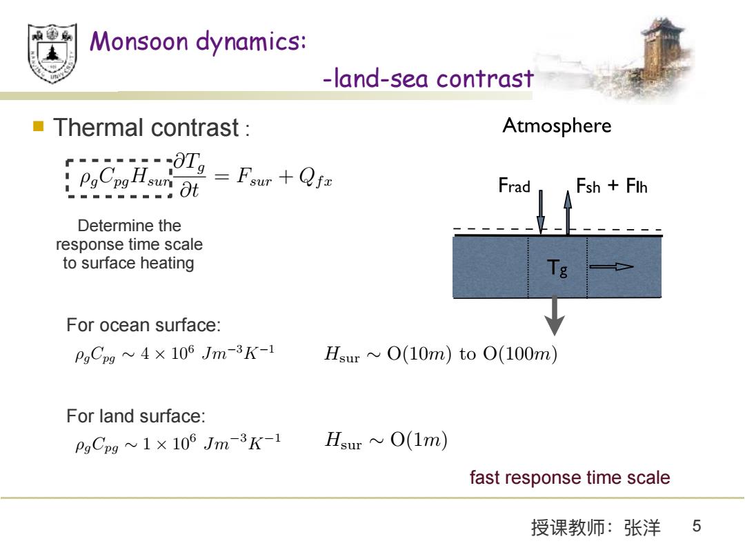
Monsoon dynamics: -land-sea contrast ■Thermal contrast: Atmosphere -月0La=Fur+Q PgCpg 1---。8t Frad Fsh Flh Determine the ( response time scale to surface heating For ocean surface: PgCpg~4×106Jm-3K-1 Hsur ~O(10m)to O(100m) For land surface: PgCpg~1x 106 Jm-3K-1 Hsur O(1m) fast response time scale 授课教师：张洋5授课教师：张洋 5 Monsoon dynamics: -land-sea contrast n Thermal contrast : 2.3 Underlying surface 2.3.1 Governing equation The tendency of the underlying surface temperature, Tg, is calculated from the energy budget equation of the surface layer: ￾gCpgHsur ⌅Tg ⌅t = Fsur + Qfx, (2.13) where ￾g is the density of the surface materials, i.e., soil density or sea water density in the ocean mixed layer, and is constant in the model; Cpg is its specific heat; Hsur is the depth of the surface layer; Fsur is the heat flux across the air- surface interface (define the flux from the atmosphere into the surface as positive), Qfx represents the e￾ect of the convergence of the horizontal heat transport and the possible heat flow into the surface layer from deeper layers. In this study, we assume the underlying surface in the standard coupled run is an ocean surface, and ￾gCpg ⇤ 4 ⇥ 106 Jm￾3K￾1. Even though the depth of the ocean mixed layer has large spatial and seasonal variation (Levitus, 1994), for simplicity we assume Hsur a constant in the model. In the transient response experiments in Section 6.1.2 and 6.3.2, we use a shallower surface layer with Hsur = 5 m as the default value. In the midlatitude, ocean mixed layer is typically 100 m in the winter and 20 m in the summer. However, we find that even with a shallow ocean mixed layer, the surface response time scale, which is around hundreds of days, is already much longer than the atmospheric response time scales and the mechanism through which the coupled system reaches the equilibrium is the same. To save the computation time, a shallower surface depth is used. Fsur has three components: radiative flux into the surface Frad, sensible heat flux from the surface to the atmosphere Fsh, which has the same definition as in Equation 2.6, and latent heat flux from the surface to the atmosphere Flh, Fsur = Frad ￾ Fsh ￾ Flh. (2.14) 54 Hsur ⇠ O(10m) to O(100m) 2.3 Underlying surface 2.3.1 Governing equation The tendency of the underlying surface temperature, Tg, is calculated from the energy budget equation of the surface layer: ￾gCpgHsur ⌅Tg ⌅t = Fsur + Qfx, (2.13) where ￾g is the density of the surface materials, i.e., soil density or sea water density in the ocean mixed layer, and is constant in the model; Cpg is its specific heat; Hsur is the depth of the surface layer; Fsur is the heat flux across the air- surface interface (define the flux from the atmosphere into the surface as positive), Qfx represents the e￾ect of the convergence of the horizontal heat transport and the possible heat flow into the surface layer from deeper layers. In this study, we assume the underlying surface in the standard coupled run is an ocean surface, and ￾gCpg ⇤ 4 ⇥ 106 Jm￾3K￾1. Even though the depth of the ocean mixed layer has large spatial and seasonal variation (Levitus, 1994), for simplicity we assume Hsur a constant in the model. In the transient response experiments in Section 6.1.2 and 6.3.2, we use a shallower surface layer with Hsur = 5 m as the default value. In the midlatitude, ocean mixed layer is typically 100 m in the winter and 20 m in the summer. However, we find that even with a shallow ocean mixed layer, the surface response time scale, which is around hundreds of days, is already much longer than the atmospheric response time scales and the mechanism through which the coupled system reaches the equilibrium is the same. To save the computation time, a shallower surface depth is used. Fsur has three components: radiative flux into the surface Frad, sensible heat flux from the surface to the atmosphere Fsh, which has the same definition as in Equation 2.6, and latent heat flux from the surface to the atmosphere Flh, Fsur = Frad ￾ Fsh ￾ Flh. (2.14) 54 For ocean surface: Determine the response time scale to surface heating ⇢gCpg ⇠ 1 ⇥ 106 Jm￾3K￾1 Hsur ⇠ O(1m) For land surface: The role of boundary layer processes in baroclinic eddy equilibration in a simple atmosphere-slab ocean coupled model Yang Zhang1 , Peter H. Stone1 1 EAPS, Massachusetts Institute of Technology, Cambridge, Massachusetts, USA. yangzh@mit.edu Introduction To understand the role of baroclinic eddies in atmospheric circulation, several theories have been proposed. However, these theories either fail to work in the boundary layer or simply neglect the influence of boundary layer processes. The study of Zhang et.al. (2009, JAS) found that, under fixed SST boundary condition, the boundary layer thermal diffusion, along with the surface heat flux, is primarily responsible for limiting PV homogenization by baroclinic ed￾dies in the boundary layer, which also provides an explanation for why the baroclinic adjustment theory does not work well there. In this study, the differ￾ent roles of different boundary layer processes in eddy equilibration are further investigated in a simple air-sea coupled model. Model Setup The atmospheric model is a modified !-plane multilevel quasi-geostrophic channel model with an interactive stratification and a simplified parameteri￾zation of atmospheric boundary layer physics, similar to that of Solomon and Stone (2001). The model has a channel length of 21040 km, a channel width of 10000 km. In this study, the horizontal resolution is 330 km and there are 17 equally spaced pressure levels in the model. A slab surface model is used to couple with the atmospheric model. The slab surface model has a fixed depth Hsur and only allows the heat exchanges with the atmosphere to influence the underlying surface temperature Tg directly. The dynamic heat transport in the ocean is simply represented by a pre-specified Q-flux. "gCpgHsur #Tg #t = Frad +Flh +Fsh +Qf x, (1) In the coupled model, the surface temperature can influence the atmospheric flow in two ways: • it is the bottom boundary condition of the atmospheric model, which can be quickly ‘felt’ by the lower level atmosphere; • the target state temperature $e in the Newtonian cooling term is set to $e(y, p,t) = $∗ e (T∗ g (y,t)) + $e xy(%rce(p,t)), thus Tg influences the radiative￾convective heating exerted on the atmospheric flow. Spin-up of the coupled model −5000 −4000 −3000 −2000 −1000 0 1000 2000 3000 4000 5000 −50 −40 −30 −20 −10 0 10 20 30 40 Latitudal Distribution of Tg* (Spinup) K (Temperature) Latitude (km) Clima. Sym.Run Eddyrun Q&Eddy warm cold surface Atmosphere Fsh eddy mixing dT>0 warm cold surface Atmosphere dT<0 Fsh d Fsh > 0 d Fsh < 0 2D symmetric run without Q-flux −5000 −4000 −3000 −2000 −1000 0 1000 2000 3000 4000 5000 −150 −100 −50 0 50 100 150 Latitude (km) W/m2 Rad. LH SH sum Eddy included run without Q-flux −5000 −4000 −3000 −2000 −1000 0 1000 2000 3000 4000 5000 −150 −100 −50 0 50 100 150 Latitude (km) W/m2 Rad. LH SH sum Eddy included run with Q-flux −5000 −4000 −3000 −2000 −1000 0 1000 2000 3000 4000 5000 −150 −100 −50 0 50 100 150 Latitude (km) W/m2 Rad. LH SH Q−fx Rs sum Figure 1: Latitudinal distribution of the underlying surface temperature in the (a) 2D symmetric run with￾out Q-flux, in the (b) eddy included run without Q-flux and in the (c) eddy included run with Q-flux compared with the climatological surface temperature (left), and the latitudinal distribution of each surface energy flux in the equilibrium state in the three simulations. Baroclinic eddies, by mixing the surface air temperature, enhance Fsh and results in smaller temperature gradient. Surface heat flux −25 −20 −15 −10 −5 0 5 200 300 400 500 600 700 800 900 1000 dT/dy pressure (mb) K/1000 km rce−sd sd,cd=0.03 rce−tcd0 tcd=0.00 rce−tcd1 tcd=0.01 rce−tcd6 tcd=0.06 0 2 4 6 8 10 12 100 200 300 400 500 600 700 800 900 1000 d[$]/dz (Full evorun) pressure (mb) K/km rce sd,cd=0.03 tcd=0.00 tcd=0.01 tcd=0.06 −150 −100 −50 0 50 100 700 750 800 850 900 950 ! Pressure (hpa) dPV/(!*dy) rce sd,cd=0.03 tcd=0.00 tcd=0.01 tcd=0.06 0 5 10 15 20 25 30 35 40 0 100 200 300 400 500 600 700 800 900 1000 pressure (mb) K Pa/s Eddy medional heat flux[v*T*](full evorun) sd,cd=0.03 tcd=0.00 tcd=0.01 tcd=0.06 Figure 2: (a) Zonal mean temperature gradient, (b) stratification, (c) PV gradient in the boundary layer and (d) poleward eddy heat flux in the cdt = 0, 0.01, 0.06 ms−1 runs and the SD runs. For the equilibrium state thermal structure, the direct influence of the latent heat flux is dominant. However, the net effect is still damping the lower atmosphere PV mixing. −10 −10 −10 −10 −10 −8 −8 −8 −8 −8 −8 −6 −6 −6 −6 −6 −6 −6 −4 −4 −4 −4 −4 −4 −4 −2 −2 −2 0 0 0 0 2 2 2 2 2 2 2 4 4 4 4 4 4 4 −2 −2 −2 6 6 6 6 6 6 6 8 8 8 −10 10 8 2 4 Latitude (km) Day 100 101 102 −2000 0 2000 −50 −30 −20 −10 −10 −10 0 0 0 10 10 10 10 10 10 −10 −10 20 30 40 50 Latitude (km) Day 100 101 102 −2000 0 2000 −8 −8 −8 −8 −8 −8 −6 −6 −6 −6 −6 −6 −6 −6 −4 −4 −4 −4 −4 −2 0 −2 0 −2 −2 0 0 2 4 2 2 4 4 6 6 6 8 8 8 8 10 10 10 Latitude (km) Day 100 101 102 −2000 0 2000 −7 −7 −7 −6 −6 −6 −5 −5 −5 −4 −4 −4 −4 −3 −3 −3 −3 −2 −2 −2 −2 −1 −1 −1 −1 0 0 0 0 1 1 1 1 2 2 2 2 3 3 3 4 4 4 4 5 5 5 5 6 6 6 7 7 7 8 8 8 9 9 Latitude (km) Day 100 101 102 −2000 0 2000 Figure 3: Transient response of Fsh − Fsh sd, Flh − Flh sd, Frad − Frad sd and Tg − Tg sd (from upper to lower pannels) when suddenly increasing the surface heat drag coefficient, where Hsur = 5m. Surface friction −20 −15 −10 −5 0 5 200 300 400 500 600 700 800 900 1000 dT/dy pressure (mb) K/1000 km rce−sd sd,cdf=0.03 rce−fcd1 cdf=0.01 rce−fcd6 cdf=0.06 −200 −150 −100 −50 0 50 100 150 700 750 800 850 900 950 ! Pressure (hpa) dPV/(!*dy) sd,cdf=0.03 cdf=0.01 cdf=0.06 0 5 10 15 20 25 0 100 200 300 400 500 600 700 800 900 1000 pressure (hpa) K m/s Poleward eddy heat flux[v*T*] sd,cdf=0.03 cdf=0.01 cdf=0.06 Figure 4: (a) Zonal mean temperature gradient, (b)PV gradient in the boundary layer and (c) poleward eddy heat flux in the cd f = 0.01, 0.06 ms−1 runs and the SD runs. Surface friction influences the equilibrium state thermal structure by modifying the eddy activities. −4 −4 −2 −2 −2 −2 −2 −2 −2 −2 −2 0 0 0 0 0 0 0 0 2 2 2 2 2 2 2 2 2 2 2 −4 −4 −4 −4 4 4 −6 −6 −4 −4 4 4 4 4 4 4 6 4 −4 6 8 4 8 −6 −6 4 −8 4 6 10 −8 0 6 −4 −10 −6 12 4 0 −4 4 −6 −8 4 −6 4 14 −12 2 −6 8 −4 6 6 4 −2 8 6 −6 −8 2 −6 4 4 4 10 6 6 −8 6 6 4 −8 6 −6 4 −2 0 0 −8 6 2 2 4 4 2 6 6 6 2 0 2 0 0 Latitude (km) Day 100 101 102 −2000 0 2000 −6 −6 −4 −4 −4 −4 −4 −4 −2 −2 −2 −2 0 −2 −2 −2 0 0 0 2 2 2 2 2 2 2 4 4 4 4 4 4 4 6 6 6 6 6 6 6 8 8 −4 2 8 8 0 8 8 8 8 8 8 8 Latitude (km) Day 100 101 102 −2000 0 2000 −2 −2 −2 −2 −1 −1 −1 −1 −1 0 0 0 0 0 1 1 1 1 1 1 2 2 2 2 2 2 3 3 3 3 −2 Latitude (km) Day 100 101 102 −2000 0 2000 −2 −2 −2 −2 0 0 0 0 2 2 2 2 2 2 −2 −2 −2 −2 2 2 2 4 4 −2 4 −4 2 4 4 2 −4 −4 −4 4 4 −4 4 4 4 0 −4 2 2 Latitude (km) Day 100 101 102 −2000 0 2000 Figure 5: Same as Fig.3 but the transient re￾sponse when suddenly reducing the surface friction. Transient response in Figs. 3 and 5 indicates three adjustment time scales in the coupled system: a quick forc￾ing time scale of the boundary layer heat flux on the lower atmosphere (∼ 1 day), a synoptic adjustment time scale of the baroclinic eddies to the zonal flow (a few days) and a much longer response time scale of the underly￾ing surface to the surface heat flux, which depends on Hsur. Under a shal￾low ocean mixed layer (5 m), this time scale is a few hundreds of days. Conclusions • Eddy mixing of the surface air potential temperature enhances the sensible heat flux, which can result in weaker meridional temperature gradient in the equilibrium state. • Since the latent heat flux is the dominant component in balancing the merid￾ional contrast of the solar radiation, reducing surface heat drag coefficient results in much stronger surface and atmospheric temperature gradients. •Reducing surface friction increases the poleward eddy heat flux in the atmo￾sphere, thus a weaker surface temperature gradient is obtained. • Surface friction and surface heat flux, in spite of their effects on the surface temperature, still act to damp the lower atmosphere PV homogenization. • The transient response of the coupled system to change in surface friction and surface heat flux displays three different time scales affecting the equilibration of the coupled model. fast response time scale