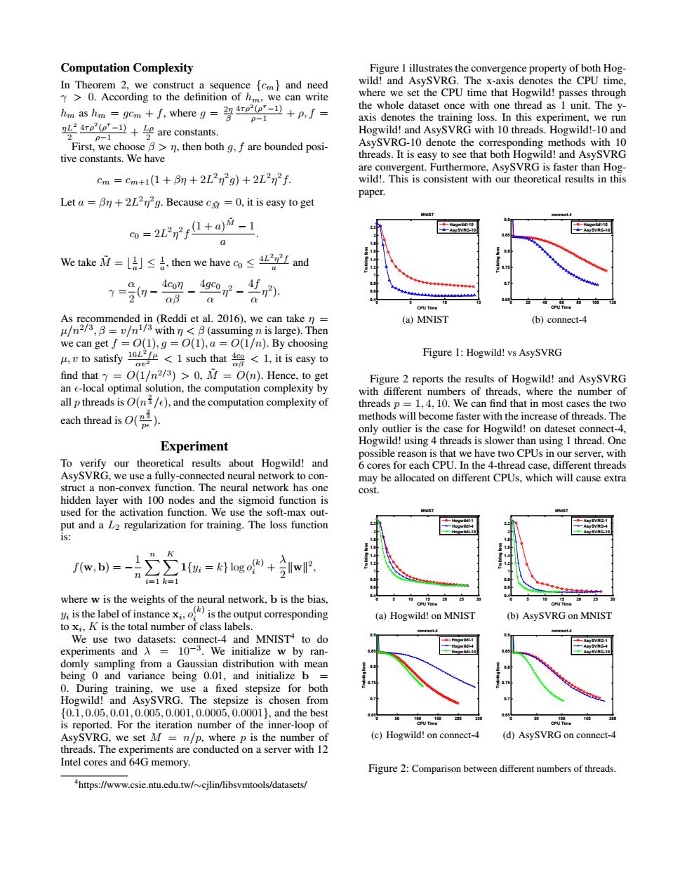
Computation Complexity Figure 1 illustrates the convergence property of both Hog- In Theorem 2,we construct a sequence [cm}and need wild!and AsySVRG.The x-axis denotes the CPU time, Y>0.According to the definition of hm,we can write where we set the CPU time that Hogwild!passes through ho as h-gem+whereg the whole dataset once with one thread as 1 unit.The y- p-1 axis denotes the training loss.In this experiment,we run are constants. Hogwild!and AsySVRG with 10 threads.Hogwild!-10 and 2 0- First,we choose B>n,then both g,f are bounded posi- AsySVRG-10 denote the corresponding methods with 10 tive constants.We have threads.It is easy to see that both Hogwild!and AsySVRG are convergent.Furthermore,AsySVRG is faster than Hog- cm=cm+1(1+6m+2L2n2g)+2L2n2f. wild!.This is consistent with our theoretical results in this paper. Let a Bn +2L2n2g.Because cxr =0,it is easy to get 0=2L2n2r1+a)"-1 We takeM=lJ≤&，then we have co≤4 I and 7=0-0g-4g2r-. aB Q As recommended in(Reddi et al.2016).we can take n (a)MNIST (b)connect-4 u/n23,B=v/n/withB(assuming n is large).Then we can get f=O(1),g=O(1),a =O(1/n).By choosing ,vto satisfy<1 such that<1.it is easy to Figure 1:Hogwild!vs AsySVRG find that =O(1/n2/3)>0,M =O(n).Hence,to get Figure 2 reports the results of Hogwild!and AsySVRG an e-local optimal solution,the computation complexity by with different numbers of threads,where the number of all p threads is O(n/e).and the computation complexity of threads p =1.4.10.We can find that in most cases the two each thread is). methods will become faster with the increase of threads.The only outlier is the case for Hogwild!on dateset connect-4, Experiment Hogwild!using 4 threads is slower than using 1 thread.One possible reason is that we have two CPUs in our server,with To verify our theoretical results about Hogwild!and 6 cores for each CPU.In the 4-thread case,different threads AsySVRG,we use a fully-connected neural network to con- may be allocated on different CPUs,which will cause extra struct a non-convex function.The neural network has one cost. hidden layer with 100 nodes and the sigmoid function is used for the activation function.We use the soft-max out- put and a L2 regularization for training.The loss function 1s: K 1 f(w,b)=- C∑1=kogo+w i=1k=1 where w is the weights of the neural network,b is the bias, is the label of instanceis the output corresponding (a)Hogwild!on MNIST (b)AsySVRG on MNIST to xi,K is the total number of class labels. We use two datasets:connect-4 and MNIST4 to do experiments and A =10-3.We initialize w by ran- domly sampling from a Gaussian distribution with mean being 0 and variance being 0.01,and initialize b 0.During training,we use a fixed stepsize for both Hogwild!and AsySVRG.The stepsize is chosen from {0.1,0.05,0.01,0.005,0.001,0.0005,0.0001},and the best is reported.For the iteration number of the inner-loop of AsySVRG,we set M=n/p,where p is the number of (c)Hogwild!on connect-4 (d)AsySVRG on connect-4 threads.The experiments are conducted on a server with 12 Intel cores and 64G memory. Figure 2:Comparison between different numbers of threads. "https://www.csie.ntu.edu.tw/cjlin/libsvmtools/datasets/Computation Complexity In Theorem 2, we construct a sequence {cm} and need γ > 0. According to the definition of hm, we can write hm as hm = gcm + f, where g = 2η β 4τρ2 (ρ τ −1) ρ−1 + ρ, f = ηL2 2 4τρ2 (ρ τ −1) ρ−1 + Lρ 2 are constants. First, we choose β > η, then both g, f are bounded posi￾tive constants. We have cm = cm+1(1 + βη + 2L 2 η 2 g) + 2L 2 η 2 f. Let a = βη + 2L 2η 2 g. Because cM˜ = 0, it is easy to get c0 = 2L 2 η 2 f (1 + a)M˜ − 1 a . We take M˜ = b 1 a c ≤ 1 a , then we have c0 ≤ 4L 2η 2 f a and γ = α 2 (η − 4c0η αβ − 4gc0 α η 2 − 4f α η 2 ). As recommended in (Reddi et al. 2016), we can take η = µ/n2/3 , β = v/n1/3 with η < β (assuming n is large). Then we can get f = O(1), g = O(1), a = O(1/n). By choosing µ, v to satisfy 16L 2 fµ αv2 < 1 such that 4c0 αβ < 1, it is easy to find that γ = O(1/n2/3 ) > 0, M˜ = O(n). Hence, to get an -local optimal solution, the computation complexity by all p threads is O(n 2 3 /), and the computation complexity of each thread is O( n 2 3 p ). Experiment To verify our theoretical results about Hogwild! and AsySVRG, we use a fully-connected neural network to con￾struct a non-convex function. The neural network has one hidden layer with 100 nodes and the sigmoid function is used for the activation function. We use the soft-max out￾put and a L2 regularization for training. The loss function is: f(w, b) = − 1 n Xn i=1 X K k=1 1{yi = k} log o (k) i + λ 2 kwk 2 , where w is the weights of the neural network, b is the bias, yi is the label of instance xi , o (k) i is the output corresponding to xi , K is the total number of class labels. We use two datasets: connect-4 and MNIST4 to do experiments and λ = 10−3 . We initialize w by ran￾domly sampling from a Gaussian distribution with mean being 0 and variance being 0.01, and initialize b = 0. During training, we use a fixed stepsize for both Hogwild! and AsySVRG. The stepsize is chosen from {0.1, 0.05, 0.01, 0.005, 0.001, 0.0005, 0.0001}, and the best is reported. For the iteration number of the inner-loop of AsySVRG, we set M = n/p, where p is the number of threads. The experiments are conducted on a server with 12 Intel cores and 64G memory. 4 https://www.csie.ntu.edu.tw/∼cjlin/libsvmtools/datasets/ Figure 1 illustrates the convergence property of both Hog￾wild! and AsySVRG. The x-axis denotes the CPU time, where we set the CPU time that Hogwild! passes through the whole dataset once with one thread as 1 unit. The y￾axis denotes the training loss. In this experiment, we run Hogwild! and AsySVRG with 10 threads. Hogwild!-10 and AsySVRG-10 denote the corresponding methods with 10 threads. It is easy to see that both Hogwild! and AsySVRG are convergent. Furthermore, AsySVRG is faster than Hog￾wild!. This is consistent with our theoretical results in this paper. 0 5 10 15 0.4 0.6 0.8 1 1.2 1.4 1.6 1.8 2 2.2 CPU Time Training loss MNIST Hogwild!-10 AsySVRG-10 (a) MNIST 0 20 40 60 80 100 120 0.65 0.7 0.75 0.8 0.85 0.9 CPU Time Training loss connect-4 Hogwild!-10 AsySVRG-10 (b) connect-4 Figure 1: Hogwild! vs AsySVRG Figure 2 reports the results of Hogwild! and AsySVRG with different numbers of threads, where the number of threads p = 1, 4, 10. We can find that in most cases the two methods will become faster with the increase of threads. The only outlier is the case for Hogwild! on dateset connect-4, Hogwild! using 4 threads is slower than using 1 thread. One possible reason is that we have two CPUs in our server, with 6 cores for each CPU. In the 4-thread case, different threads may be allocated on different CPUs, which will cause extra cost. 0 5 10 15 20 25 30 0.4 0.6 0.8 1 1.2 1.4 1.6 1.8 2 2.2 CPU Time Training loss MNIST Hogwild!-1 Hogwild!-4 Hogwild!-10 (a) Hogwild! on MNIST 0 5 10 15 20 25 30 0.4 0.6 0.8 1 1.2 1.4 1.6 1.8 2 2.2 CPU Time Training loss MNIST AsySVRG-1 AsySVRG-4 AsySVRG-10 (b) AsySVRG on MNIST 0 50 100 150 200 250 0.65 0.7 0.75 0.8 0.85 0.9 CPU Time Training loss connect-4 Hogwild!-1 Hogwild!-4 Hogwild!-10 (c) Hogwild! on connect-4 0 50 100 150 200 0.65 0.7 0.75 0.8 0.85 0.9 CPU Time Training loss connect-4 AsySVRG-1 AsySVRG-4 AsySVRG-10 (d) AsySVRG on connect-4 Figure 2: Comparison between different numbers of threads