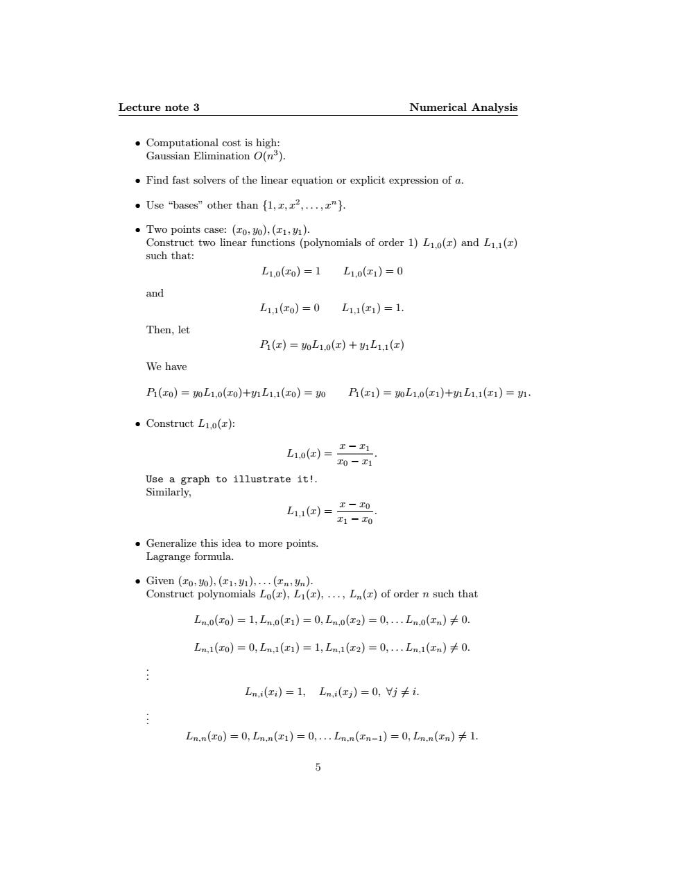
Lecture note 3 Numerical Analysis Computational cost is high: Gaussian Elimination O(n3). Find fast solvers of the linear equation or explicit expression of a. 。Use“bases'”other than{L,x,z2,,z}. .Two points case:(To,y0),(x1,21). Construct two linear functions (polynomials of order 1)L1.o(z)and L11(x) such that: L1.0(z0)=1L1.0(x1)=0 and L1,1(xo)=0L1,1(x1)=1. Then,let 乃(x)=0L1,o(x)+hL1,1(x) We have P1(xo)=0L1,0(xo)+y1L1,1(x0)=0 (c1)=0L1,0(x1)+1L1,1(x1)=h. ·Construct L1,o(r): L1.0(a)=工- T0-E1 Use a graph to illustrate it!. Similarly, L1,1()=-0 x1一T0 Generalize this idea to more points. Lagrange formula. .Given (To,20),(1:11),...(In:Un). Construct polynomials Lo(x),L1(),...,Ln(x)of order n such that Ln.o(o)=1,Ln.o(1)=0,Ln.o(2)=0,...In.o(n)0. Ln,1(xo)=0,Ln,1(x1)=1,Lm,1(x2）=0,.Ln,1(xn)≠0. Ln.i(xi)=1,Ln.i(j)=0,Vj#i. Ln.n(0)=0,Ln,n(1)=0,...Ln.n(In-1)=0,Ln,n(n)#1. 5Lecture note 3 Numerical Analysis • Computational cost is high: Gaussian Elimination O(n 3 ). • Find fast solvers of the linear equation or explicit expression of a. • Use “bases” other than {1, x, x2 , . . . , xn}. • Two points case: (x0, y0),(x1, y1). Construct two linear functions (polynomials of order 1) L1,0(x) and L1,1(x) such that: L1,0(x0) = 1 L1,0(x1) = 0 and L1,1(x0) = 0 L1,1(x1) = 1. Then, let P1(x) = y0L1,0(x) + y1L1,1(x) We have P1(x0) = y0L1,0(x0)+y1L1,1(x0) = y0 P1(x1) = y0L1,0(x1)+y1L1,1(x1) = y1. • Construct L1,0(x): L1,0(x) = x − x1 x0 − x1 . Use a graph to illustrate it!. Similarly, L1,1(x) = x − x0 x1 − x0 . • Generalize this idea to more points. Lagrange formula. • Given (x0, y0),(x1, y1), . . .(xn, yn). Construct polynomials L0(x), L1(x), . . . , Ln(x) of order n such that Ln,0(x0) = 1, Ln,0(x1) = 0, Ln,0(x2) = 0, . . . Ln,0(xn) 6= 0. Ln,1(x0) = 0, Ln,1(x1) = 1, Ln,1(x2) = 0, . . . Ln,1(xn) 6= 0. . . . Ln,i(xi) = 1, Ln,i(xj ) = 0, ∀j 6= i. . . . Ln,n(x0) = 0, Ln,n(x1) = 0, . . . Ln,n(xn−1) = 0, Ln,n(xn) 6= 1. 5