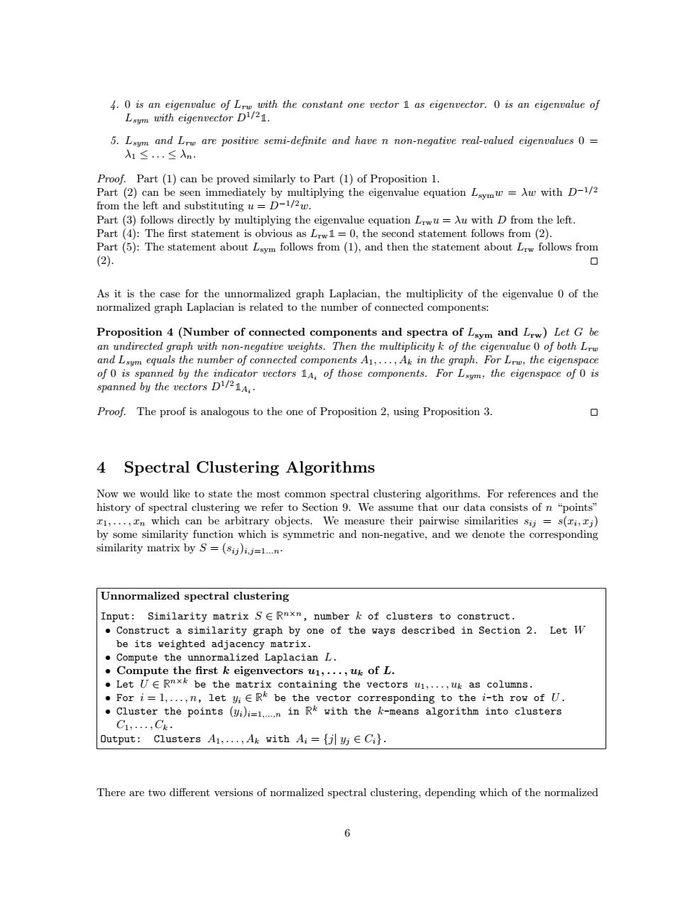
4.0 is an eigenvalue of Lrw with the constant one vector 1 as eigenvector.0 is an eigenvalue of Lsym with eigenvector D1/21. 5.Lsym and Lrw are positive semi-definite and have n non-negative real-valued eigenvalues 0= 入1≤.≤入n Proof.Part(1)can be proved similarly to Part (1)of Proposition 1. Part (2)can be seen immediately by multiplying the eigenvalue equation Lsymw=Aw with D-1/2 from the left and substituting u=D-1/2w. Part (3)follows directly by multiplying the eigenvalue equation Lrwu=Au with D from the left. Part (4):The first statement is obvious as Lrw1=0,the second statement follows from(2). Part(5):The statement about Lsym follows from (1),and then the statement about Lrw follows from (2) As it is the case for the unnormalized graph Laplacian,the multiplicity of the eigenvalue 0 of the normalized graph Laplacian is related to the number of connected components: Proposition 4(Number of connected components and spectra of Lsym and Lw)Let G be an undirected graph with non-negative weights.Then the multiplicity k of the eigenvalue O of both Lrw and Lsum equals the number of connected components A1,...,Ak in the graph.For Lrw;the eigenspace of 0 is spanned by the indicator vectors 1A.of those components.For Lsym,the eigenspace of 0 is spanned by the vectors D21A. Proof.The proof is analogous to the one of Proposition 2,using Proposition 3. 0 4 Spectral Clustering Algorithms Now we would like to state the most common spectral clustering algorithms.For references and the history of spectral clustering we refer to Section 9.We assume that our data consists of n "points" x1,...,In which can be arbitrary objects.We measure their pairwise similarities sij=s(ri,zj) by some similarity function which is symmetric and non-negative,and we denote the corresponding similarity matrix by S=(sij)i.j=1...n. Unnormalized spectral clustering Input:Similarity matrix SE Rnxm,number k of clusters to construct. Construct a similarity graph by one of the ways described in Section 2.Let W be its weighted adjacency matrix. Compute the unnormalized Laplacian L. Compute the first k eigenvectors u1,...,uk of L. Let UE Rnxk be the matrix containing the vectors u1,...,uk as columns. For i=1,...,n,let yi E R be the vector corresponding to the i-th row of U. .Cluster the points ()i=1..n in Rk with the k-means algorithm into clusters C1,,Ck· Output: Clusters A1,...,Ak with Ai={jl y E Ci}. There are two different versions of normalized spectral clustering,depending which of the normalized 64. 0 is an eigenvalue of Lrw with the constant one vector ✶ as eigenvector. 0 is an eigenvalue of Lsym with eigenvector D1/2✶. 5. Lsym and Lrw are positive semi-definite and have n non-negative real-valued eigenvalues 0 = λ1 ≤ . . . ≤ λn. Proof. Part (1) can be proved similarly to Part (1) of Proposition 1. Part (2) can be seen immediately by multiplying the eigenvalue equation Lsymw = λw with D−1/2 from the left and substituting u = D−1/2w. Part (3) follows directly by multiplying the eigenvalue equation Lrwu = λu with D from the left. Part (4): The first statement is obvious as Lrw✶ = 0, the second statement follows from (2). Part (5): The statement about Lsym follows from (1), and then the statement about Lrw follows from (2). 2 As it is the case for the unnormalized graph Laplacian, the multiplicity of the eigenvalue 0 of the normalized graph Laplacian is related to the number of connected components: Proposition 4 (Number of connected components and spectra of Lsym and Lrw) Let G be an undirected graph with non-negative weights. Then the multiplicity k of the eigenvalue 0 of both Lrw and Lsym equals the number of connected components A1, . . . , Ak in the graph. For Lrw, the eigenspace of 0 is spanned by the indicator vectors ✶Ai of those components. For Lsym, the eigenspace of 0 is spanned by the vectors D1/2✶Ai . Proof. The proof is analogous to the one of Proposition 2, using Proposition 3. 2 4 Spectral Clustering Algorithms Now we would like to state the most common spectral clustering algorithms. For references and the history of spectral clustering we refer to Section 9. We assume that our data consists of n “points” x1, . . . , xn which can be arbitrary objects. We measure their pairwise similarities sij = s(xi , xj ) by some similarity function which is symmetric and non-negative, and we denote the corresponding similarity matrix by S = (sij )i,j=1...n. Unnormalized spectral clustering Input: Similarity matrix S ∈ ❘ n×n, number k of clusters to construct. • Construct a similarity graph by one of the ways described in Section 2. Let W be its weighted adjacency matrix. • Compute the unnormalized Laplacian L. • Compute the first k eigenvectors u1, . . . , uk of L. • Let U ∈ ❘ n×k be the matrix containing the vectors u1, . . . , uk as columns. • For i = 1, . . . , n, let yi ∈ ❘ k be the vector corresponding to the i-th row of U. • Cluster the points (yi)i=1,...,n in ❘ k with the k-means algorithm into clusters C1, . . . , Ck. Output: Clusters A1, . . . , Ak with Ai = {j| yj ∈ Ci}. There are two different versions of normalized spectral clustering, depending which of the normalized 6