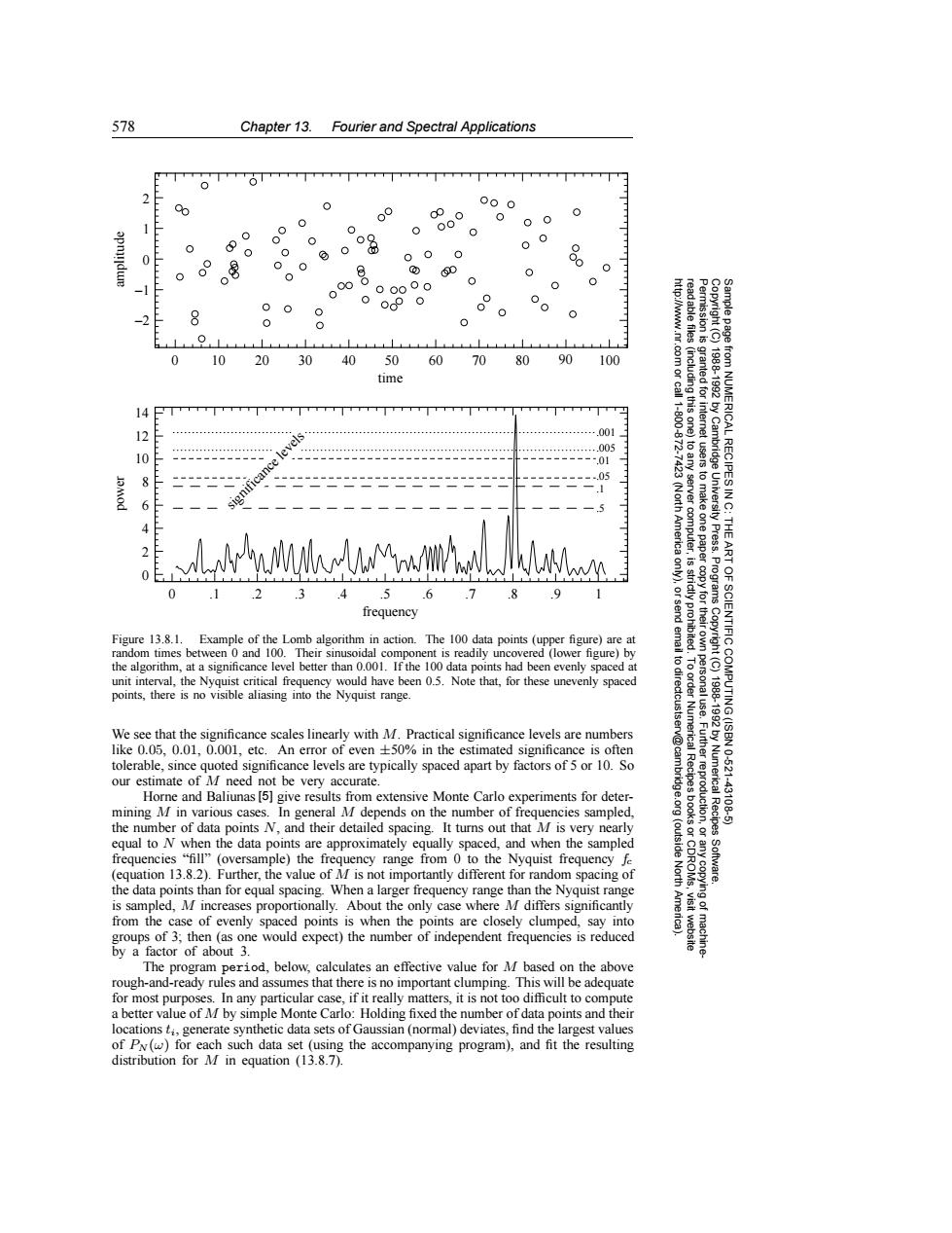
578 Chapter 13.Fourier and Spectral Applications T 0 01 2 00 000 0 0 0 0 1 00 00 00 0 0 00 0 00 0 0 0 00 0 -1 00000 0 0 0 0 00 0c9 0 2 8 0 0 0 0 Permission is 0 10 20 30 40 50 60 70 80 90 100 83 time 14 11-600 (including this one) granted for ….001 .005 10 ------.01 8 .05 6 (North America to any server computer, tusers to make one paper 1988-1992 by Cambridge University Press. from NUMERICAL RECIPES IN C: THE 2 是 ART 0 .1 .2 3 4 .5 .6 .7 8 .9 1 Programs frequency send copy for their Figure 13.8.1. Example of the Lomb algorithm in action.The 100 data points(upper figure)are at random times between 0 and 100.Their sinusoidal component is readily uncovered (lower figure)by the algorithm,at a significance level better than 0.001.If the 100 data points had been evenly spaced at to dir Copyright(C) unit interval,the Nyquist critical frequency would have been 0.5.Note that,for these unevenly spaced points,there is no visible aliasing into the Nyquist range. ectcustser We see that the significance scales linearly with M.Practical significance levels are numbers 1988-1992 by Numerical Recipes OF SCIENTIFIC COMPUTING(ISBN 0-521- like 0.05,0.01,0.001,etc.An error of even +50%in the estimated significance is often v@cam tolerable,since quoted significance levels are typically spaced apart by factors of 5 or 10.So our estimate of M need not be very accurate. Horne and Baliunas [5]give results from extensive Monte Carlo experiments for deter- mining M in various cases.In general M depends on the number of frequencies sampled, -431085 the number of data points N,and their detailed spacing.It turns out that M is very nearly equal to N when the data points are approximately equally spaced,and when the sampled (outside frequencies "fill"(oversample)the frequency range from 0 to the Nyquist frequency fe (equation 13.8.2).Further,the value of M is not importantly different for random spacing of North Software. the data points than for equal spacing.When a larger frequency range than the Nyquist range is sampled,M increases proportionally.About the only case where M differs significantly from the case of evenly spaced points is when the points are closely clumped,say into groups of 3;then(as one would expect)the number of independent frequencies is reduced visit website by a factor of about 3. The program period,below,calculates an effective value for M based on the above rough-and-ready rules and assumes that there is no important clumping.This will be adequate for most purposes.In any particular case,if it really matters,it is not too difficult to compute a better value of M by simple Monte Carlo:Holding fixed the number of data points and their locations ti,generate synthetic data sets of Gaussian(normal)deviates,find the largest values of P(w)for each such data set(using the accompanying program),and fit the resulting distribution for M in equation (13.8.7).578 Chapter 13. Fourier and Spectral Applications Permission is granted for internet users to make one paper copy for their own personal use. Further reproduction, or any copyin Copyright (C) 1988-1992 by Cambridge University Press. Programs Copyright (C) 1988-1992 by Numerical Recipes Software. Sample page from NUMERICAL RECIPES IN C: THE ART OF SCIENTIFIC COMPUTING (ISBN 0-521-43108-5) g of machine￾readable files (including this one) to any server computer, is strictly prohibited. To order Numerical Recipes books or CDROMs, visit website http://www.nr.com or call 1-800-872-7423 (North America only), or send email to directcustserv@cambridge.org (outside North America). −2 −1 0 1 2 0 10 20 30 40 50 60 70 80 90 100 time amplitude .001 .005 .01 .05 .1 .5 0 2 4 6 8 10 12 14 power 0 .1 .2 .3 .4 .5 .6 .7 .8 .9 1 frequency significance levels Figure 13.8.1. Example of the Lomb algorithm in action. The 100 data points (upper figure) are at random times between 0 and 100. Their sinusoidal component is readily uncovered (lower figure) by the algorithm, at a significance level better than 0.001. If the 100 data points had been evenly spaced at unit interval, the Nyquist critical frequency would have been 0.5. Note that, for these unevenly spaced points, there is no visible aliasing into the Nyquist range. We see that the significance scales linearly with M. Practical significance levels are numbers like 0.05, 0.01, 0.001, etc. An error of even ±50% in the estimated significance is often tolerable, since quoted significance levels are typically spaced apart by factors of 5 or 10. So our estimate of M need not be very accurate. Horne and Baliunas [5] give results from extensive Monte Carlo experiments for deter￾mining M in various cases. In general M depends on the number of frequencies sampled, the number of data points N, and their detailed spacing. It turns out that M is very nearly equal to N when the data points are approximately equally spaced, and when the sampled frequencies “fill” (oversample) the frequency range from 0 to the Nyquist frequency fc (equation 13.8.2). Further, the value of M is not importantly different for random spacing of the data points than for equal spacing. When a larger frequency range than the Nyquist range is sampled, M increases proportionally. About the only case where M differs significantly from the case of evenly spaced points is when the points are closely clumped, say into groups of 3; then (as one would expect) the number of independent frequencies is reduced by a factor of about 3. The program period, below, calculates an effective value for M based on the above rough-and-ready rules and assumes that there is no important clumping. This will be adequate for most purposes. In any particular case, if it really matters, it is not too difficult to compute a better value of M by simple Monte Carlo: Holding fixed the number of data points and their locations ti, generate synthetic data sets of Gaussian (normal) deviates, find the largest values of PN (ω) for each such data set (using the accompanying program), and fit the resulting distribution for M in equation (13.8.7)