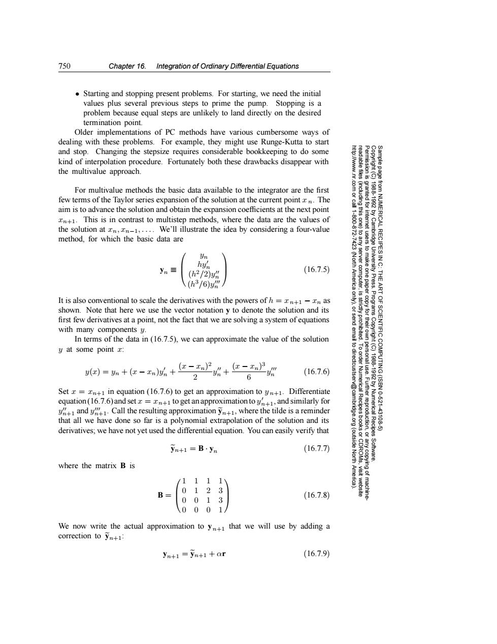
750 Chapter 16.Integration of Ordinary Differential Equations .Starting and stopping present problems.For starting,we need the initial values plus several previous steps to prime the pump.Stopping is a problem because equal steps are unlikely to land directly on the desired termination point. Older implementations of PC methods have various cumbersome ways of dealing with these problems.For example,they might use Runge-Kutta to start and stop.Changing the stepsize requires considerable bookkeeping to do some kind of interpolation procedure.Fortunately both these drawbacks disappear with the multivalue approach. For multivalue methods the basic data available to the integrator are the first few terms of the Taylor series expansion of the solution at the current point xn.The aim is to advance the solution and obtain the expansion coefficients at the next point n+1.This is in contrast to multistep methods,where the data are the values of 遠分 the solution at,,....We'll illustrate the idea by considering a four-value method,for which the basic data are RECIPES yn 4 2 hyn yn目 (h2/2)yh (16.7.5) (h3/6) It is also conventional to scale the derivatives with the powers ofh=n+1-n as shown.Note that here we use the vector notation y to denote the solution and its 9 first few derivatives at a point,not the fact that we are solving a system ofequations 分、02◆ with many components y. In terms of the data in(16.7.5),we can approximate the value of the solution 6 y at some point x: 2h+包-小3 @=如+e-M+在-， (16.7.6) 6 Set z =n+1 in equation (16.7.6)to get an approximation to yn+1.Differentiate equation(16.7.6)and set=n+1to get anapproximation toyn,and similarly for umerical 10.621 and y Call the resulting approximation y,where the tilde is a reminder that all we have done so far is a polynomial extrapolation of the solution and its 431 derivatives;we have not yet used the differential equation.You can easily verify that Recipes yn+1=B.yn (16.7.7) where the matrix B is /1111 0 1 2 3 0 01 3 (16.7.8) 000 1 We now write the actual approximation to ythat we will use by adding a correction to yn+1: yn+1 yn+1 +ar (16.7.9)750 Chapter 16. Integration of Ordinary Differential Equations Permission is granted for internet users to make one paper copy for their own personal use. Further reproduction, or any copyin Copyright (C) 1988-1992 by Cambridge University Press. Programs Copyright (C) 1988-1992 by Numerical Recipes Software. Sample page from NUMERICAL RECIPES IN C: THE ART OF SCIENTIFIC COMPUTING (ISBN 0-521-43108-5) g of machine￾readable files (including this one) to any server computer, is strictly prohibited. To order Numerical Recipes books or CDROMs, visit website http://www.nr.com or call 1-800-872-7423 (North America only), or send email to directcustserv@cambridge.org (outside North America). • Starting and stopping present problems. For starting, we need the initial values plus several previous steps to prime the pump. Stopping is a problem because equal steps are unlikely to land directly on the desired termination point. Older implementations of PC methods have various cumbersome ways of dealing with these problems. For example, they might use Runge-Kutta to start and stop. Changing the stepsize requires considerable bookkeeping to do some kind of interpolation procedure. Fortunately both these drawbacks disappear with the multivalue approach. For multivalue methods the basic data available to the integrator are the first few terms of the Taylor series expansion of the solution at the current point x n. The aim is to advance the solution and obtain the expansion coefficients at the next point xn+1. This is in contrast to multistep methods, where the data are the values of the solution at xn, xn−1,... . We’ll illustrate the idea by considering a four-value method, for which the basic data are yn ≡   yn hy
n (h2/2)y

n (h3/6)y


n   (16.7.5) It is also conventional to scale the derivatives with the powers of h = x n+1 − xn as shown. Note that here we use the vector notation y to denote the solution and its first few derivatives at a point, not the fact that we are solving a system of equations with many components y. In terms of the data in (16.7.5), we can approximate the value of the solution y at some point x: y(x) = yn + (x − xn)y
n + (x − xn)2 2 y

n + (x − xn)3 6 y


n (16.7.6) Set x = xn+1 in equation (16.7.6) to get an approximation to y n+1. Differentiate equation (16.7.6) and set x = xn+1 to get an approximation to y
n+1, and similarly for y

n+1 and y


n+1. Call the resulting approximation yn+1, where the tilde is a reminder that all we have done so far is a polynomial extrapolation of the solution and its derivatives; we have not yet used the differential equation. You can easily verify that yn+1 = B · yn (16.7.7) where the matrix B is B =   1111 0123 0013 0001   (16.7.8) We now write the actual approximation to yn+1 that we will use by adding a correction to yn+1: yn+1 = yn+1 + αr (16.7.9)