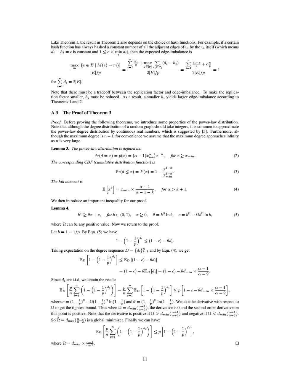
Like Theorem 1,the result in Theorem 2 also depends on the choice of hash functions.For example,if a certain hash function has always hashed a constant number of all the adjacent edges of vi by the vi itself(which means di-hi =c is constant and 1 <c<min da),then the expected edge-imbalance is maxl{e∈ElM(e)=mH +max∑(d,-h,】 可lEPy 盆+ 2E1/P =1 EV/p 2E/p ford= Note that there must be a tradeoff between the replication factor and edge-imbalance.To make the replica- tion factor smaller,hi must be reduced.As a result,a smaller hi yields larger edge-imbalance according to Theorems 1 and 2. A.3 The Proof of Theorem 3 Proof.Before proving the following theorems.we introduce some properties of the power-law distribution. Note that although the degree distribution of a random graph should take integers,it is common to approximate the power-law degree distribution by continuous real numbers,which is suggested by [5].Furthermore,al- though the maximum degree is n-1,for convenience we assume that the maximum degree approaches infinity as n is very large. Lemma 3.The power-law distribution is defined as: Pr(d=)=p()=(a-1)xmint-,for x2 Imin. (2) The corresponding CDF(cumulative distribution function)is tl-a prd≤)=F=l-aa (3) The kth moment is B=minx a1 a-1-k fora>k+1. (4) We then introduce an important inequality for our proof. Lemma 4. b-≥0z+c,forb∈(0,1)，x≥0,0=b21nb,c=b2-2 bInb, (5 where can be any positive value.Now we return to the proof. Let b =1-1/p.By Eqn.(5)we have 1-(0-)sa-g-a. Taking expectation on the degree sequence D={di and by Eqn.(4),we get 01-(-)]s-g-a =1-0-en4=1-d小-dnx&-号 Since d;are i.i.d,we obtain the result: E(--》】-空--]sl-c-a×8周引 where c=(1-1)-(1-1)In(1-1)and 0=(1-1)In(1-1).We take the derivative with respect to to get the tightest bound.Thus when=dn().the derivative is 0 and the second order derivative on this point is positive.Note that the derivative is positive ifd)and negative if<d). So =dmin (is a global minimizer.Finally we can have: E(-(-))】s-1-] where dmin x ◇ 11Like Theorem 1, the result in Theorem 2 also depends on the choice of hash functions. For example, if a certain hash function has always hashed a constant number of all the adjacent edges of vi by the vi itself (which means di − hi = c is constant and 1 ≤ c < min i di), then the expected edge-imbalance is max m |{e ∈ E | M(e) = m}| |E|/p = Pn i=1 hi p + max j∈[p] P vi∈Pj (di − hi) 2|E|/p = Pn i=1 di−c p + c n p 2|E|/p = 1 for Pn i=1 di = 2|E|. Note that there must be a tradeoff between the replication factor and edge-imbalance. To make the replica￾tion factor smaller, hi must be reduced. As a result, a smaller hi yields larger edge-imbalance according to Theorems 1 and 2. A.3 The Proof of Theorem 3 Proof. Before proving the following theorems, we introduce some properties of the power-law distribution. Note that although the degree distribution of a random graph should take integers, it is common to approximate the power-law degree distribution by continuous real numbers, which is suggested by [5]. Furthermore, al￾though the maximum degree is n−1, for convenience we assume that the maximum degree approaches infinity as n is very large. Lemma 3. The power-law distribution is defined as: Pr(d = x) = p(x) = (α − 1)x α−1 min x −α , for x ≥ xmin. (2) The corresponding CDF (cumulative distribution function) is Pr(d ≤ x) = F(x) = 1 − x 1−α x 1−α min . (3) The kth moment is E h x k i = xmin × α − 1 α − 1 − k , for α > k + 1. (4) We then introduce an important inequality for our proof. Lemma 4. b x ≥ θx + c, for b ∈ (0, 1), x ≥ 0, θ = b Ω ln b, c = b Ω − Ωb Ω ln b, (5) where Ω can be any positive value. Now we return to the proof. Let b = 1 − 1/p. By Eqn. (5) we have 1 −  1 − 1 p di ≤ (1 − c) − θdi. Taking expectation on the degree sequence D = {di} n i=1 and by Eqn. (4), we get ED  1 −  1 − 1 p di  ≤ ED [(1 − c) − θdi] = (1 − c) − θED [di] = (1 − c) − θdmin × α − 1 α − 2 . Since di are i.i.d, we obtain the result: ED " p n Xn i=1  1 −  1 − 1 p di # = p n Xn i=1 ED  1 −  1 − 1 p di  ≤ p  1 − c − θdmin × α − 1 α − 2  , where c = (1− 1 p ) Ω −Ω(1− 1 p ) Ω ln(1− 1 p ) and θ = (1− 1 p ) Ω ln(1− 1 p ). We take the derivative with respect to Ω to get the tightest bound. Thus when Ω = dmin( α−1 α−2 ), the derivative is 0 and the second order derivative on this point is positive. Note that the derivative is positive if Ω > dmin( α−1 α−2 ) and negative if Ω < dmin( α−1 α−2 ). So Ω =ˆ dmin( α−1 α−2 ) is a global minimizer. Finally we can have: ED " p n Xn i=1  1 −  1 − 1 p di # ≤ p  1 −  1 − 1 p Ωˆ  , where Ω =ˆ dmin × α−1 α−2 . 11