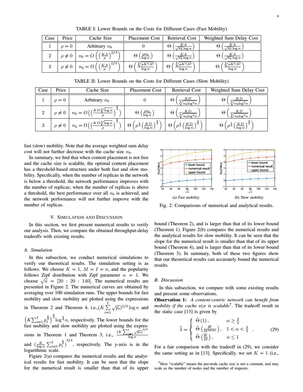
9 TABLE I:Lower Bounds on the Costs for Different Cases(Fast Mobility) Case Price Cache Size Placement Cost Retrieval Cost Weighted Sum Delay Cost 1 p=0 Arbitrary nb 0 Θ （ns log n ynslogn KA 2 p≠0 nb=O () 6(） 6(m) 9(dn) 3 p卡0 nb= 2 日 PK2A2 VPK2A2 日 PK2A2 logn logn logn TABLE II:Lower Bounds on the Costs for Different Cases (Slow Mobility) Case Price Cache Size Placement Cost Retrieval Cost Weighted Sum Delay Cost p=0 Arbitrary nb 0 KD KD nolog2元 Vntlog'n 2 p≠0 nb = O(KD@g元 6() KD KD p Vnblog2n nblog2n 3 P≠0 n=2( (KDVlog元 0 (p(品 (p() (p() fast(slow)mobility.Note that the average weighted sum delay cost will not further decrease with the cache size n. In summary,we find that when content placement is not free and the cache size is scalable,the optimal content placement ◆-lower bound -lower bound numencal resu has a threshold-based structure under both fast and slow mo- numencal result upper bound upper bound bility.Specifically,when the number of replicas in the network is below a threshold,the network performance improves with the number of replicas;when the number of replicas is above 0 100120 60 a threshold,the best performance over all n is achieved,and 10120 the network performance will not further improve with the (a)Fast mobility (b)Slow mobility number of replicas. Fig.2:Comparisons of numerical and analytical results. V.SIMULATION AND DISCUSSION In this section,we first present numerical results to verify bound (Theorem 2),and is larger than that of its lower bound our analysis.Then,we compare the obtained throughput-delay (Theorem 1).Figure 2(b)compares the numerical results and tradeoffs with existing results. the analytical results for slow mobility.It can be seen that the slope for the numerical result is smaller than that of its upper A.Simulation bound (Theorem 4),and is larger than that of its lower bound (Theorem 3).In summary,both of these two figures show In this subsection,we conduct numerical simulations to that our theoretical results can accurately bound the numerical verify our theoretical results.The simulation setting is as results. follows.We choose K=1,M=I=n,and the popularity follows Zipf distribution with Zipf parameter a 1.We choose v元=[20：20：140.The numerical results are B.Discussion presented in Figure 2.The numerical curves are obtained by In this subsection,we compare with some existing results averaging over 100 simulation runs.The upper bounds for fast and present some observations. mobility and slow mobility are plotted using the expressions Observation 1:A content-centric network can benefit from in Theorem 2 and Theorem 4.i.e.(K)2/3logn and mobility if the cache size is scalable.The tradeoff result in i=1 the static case [13]is given by epectively.The lower bounds for the 白(1)， a≥是 Doe 合(w),1<a<是. (29) ad(昏∑).repecte,Tey-asiss in the 6(), a≤1 For a fair comparison with the tradeoff in(29),we consider logarithmic scale. Figure 2(a)compares the numerical results and the analyt- the same setting as in [13].Specifically,we set K=1 (i.e., ical results for fast mobility.It can be seen that the slope for the numerical result is smaller than that of its upper 7Here"scalable"means the per-node cache size is not a constant,and may scale as the number of nodes and the number of requests.9 TABLE I: Lower Bounds on the Costs for Different Cases (Fast Mobility) Case Price Cache Size Placement Cost Retrieval Cost Weighted Sum Delay Cost 1 ρ = 0 Arbitrary nb 0 Θ € √ KA nb log n Š Θ € √ KA nb log n Š 2 ρ ̸= 0 nb = O € KA ρ Š2/3 ‹ Θ € ρnb log n Š Θ € √ KA nb log n Š Θ € √ KA nb log n Š 3 ρ ̸= 0 nb = Ω € KA ρ Š2/3 ‹ Θ √3 ρK2A2 log n ‹ Θ √3 ρK2A2 log n ‹ Θ √3 ρK2A2 log n ‹ TABLE II: Lower Bounds on the Costs for Different Cases (Slow Mobility) Case Price Cache Size Placement Cost Retrieval Cost Weighted Sum Delay Cost 1 ρ = 0 Arbitrary nb 0 Θ  KD √3 nblog2n ‹ Θ  KD √3 nblog2n ‹ 2 ρ ̸= 0 nb = O €€ KD√3 log n ρ Š 3 4 Š Θ € ρnb log n Š Θ  KD √3 nblog2n ‹ Θ  KD √3 nblog2n ‹ 3 ρ ̸= 0 nb = Ω€€ KD√3 log n ρ Š 3 4 Š Θ  ρ 1 4 € KD log n Š 3 4 ‹ Θ  ρ 1 4 € KD log n Š 3 4 ‹ Θ  ρ 1 4 € KD log n Š 3 4 ‹ fast (slow) mobility. Note that the average weighted sum delay cost will not further decrease with the cache size nb. In summary, we find that when content placement is not free and the cache size is scalable, the optimal content placement has a threshold-based structure under both fast and slow mo￾bility. Specifically, when the number of replicas in the network is below a threshold, the network performance improves with the number of replicas; when the number of replicas is above a threshold, the best performance over all nb is achieved, and the network performance will not further improve with the number of replicas. V. SIMULATION AND DISCUSSION In this section, we first present numerical results to verify our analysis. Then, we compare the obtained throughput-delay tradeoffs with existing results. A. Simulation In this subsection, we conduct numerical simulations to verify our theoretical results. The simulation setting is as follows. We choose K = 1, M = I = n, and the popularity follows Zipf distribution with Zipf parameter α = 1. We choose √ n = [20 : 20 : 140]. The numerical results are presented in Figure 2. The numerical curves are obtained by averaging over 100 simulation runs. The upper bounds for fast mobility and slow mobility are plotted using the expressions in Theorem 2 and Theorem 4, i.e.,(K P I i=1 √pi) 2/3 log n and € K PI i=1 p 2 3 i Š 3 4 log 5 4 n, respectively. The lower bounds for the fast mobility and slow mobility are plotted using the expres￾sions in Theorem 1 and Theorem 3, i.e., (K PI i=1 √pi) 2/3 log n and ( K log n PI i=1 p 2 3 i ) 3/4 , respectively. The y-axis is in the logarithmic scale. Figure 2(a) compares the numerical results and the analyt￾ical results for fast mobility. It can be seen that the slope for the numerical result is smaller than that of its upper 20 40 60 80 100 120 140 √ n 0 1 2 3 4 5 6 log(Delay) lower bound numerical result upper bound (a) Fast mobility 20 40 60 80 100 120 140 √ n -1 0 1 2 3 4 5 log(Delay) lower bound numerical result upper bound (b) Slow mobility Fig. 2: Comparisons of numerical and analytical results. bound (Theorem 2), and is larger than that of its lower bound (Theorem 1). Figure 2(b) compares the numerical results and the analytical results for slow mobility. It can be seen that the slope for the numerical result is smaller than that of its upper bound (Theorem 4), and is larger than that of its lower bound (Theorem 3). In summary, both of these two figures show that our theoretical results can accurately bound the numerical results. B. Discussion In this subsection, we compare with some existing results and present some observations. Observation 1: A content-centric network can benefit from mobility if the cache size is scalable7 . The tradeoff result in the static case [13] is given by λ¯ = 8 >< >: Θ (1) ˜ , α ≥ 3 2 Θ˜ € W¯ M3−2α Š , 1 < α < 3 2 Θ˜ € W¯ M Š , α ≤ 1 . (29) For a fair comparison with the tradeoff in (29), we consider the same setting as in [13]. Specifically, we set K = 1 (i.e., 7Here “scalable” means the per-node cache size is not a constant, and may scale as the number of nodes and the number of requests