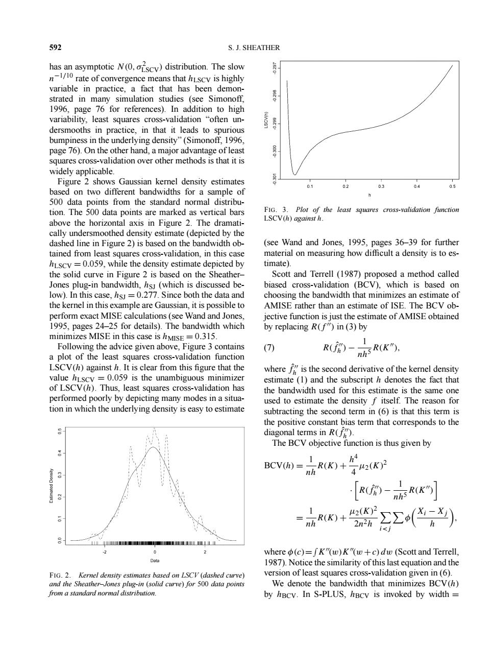
592 S.J.SHEATHER has an asymptotic N(0,scv)distribution.The slow n/1rate of convergence means that hscv is highly variable in practice,a fact that has been demon- strated in many simulation studies (see Simonoff, 8520 1996,page 76 for references).In addition to high variability,least squares cross-validation "often un- dersmooths in practice,in that it leads to spurious bumpiness in the underlying density"(Simonoff,1996, page 76).On the other hand,a major advantage of least squares cross-validation over other methods is that it is widely applicable. Figure 2 shows Gaussian kernel density estimates 0.1 02 0.3 0.4 0.5 based on two different bandwidths for a sample of 500 data points from the standard normal distribu- tion.The 500 data points are marked as vertical bars FIG.3.Plot of the least squares cross-validation function above the horizontal axis in Figure 2.The dramati- LSCV(h)against h. cally undersmoothed density estimate(depicted by the dashed line in Figure 2)is based on the bandwidth ob- (see Wand and Jones,1995,pages 36-39 for further tained from least squares cross-validation,in this case material on measuring how difficult a density is to es- hLscy =0.059,while the density estimate depicted by timate). the solid curve in Figure 2 is based on the Sheather- Scott and Terrell(1987)proposed a method called Jones plug-in bandwidth,hs(which is discussed be- biased cross-validation (BCV),which is based on low).In this case,hsJ=0.277.Since both the data and choosing the bandwidth that minimizes an estimate of the kernel in this example are Gaussian,it is possible to AMISE rather than an estimate of ISE.The BCV ob- perform exact MISE calculations(see Wand and Jones, jective function is just the estimate of AMISE obtained 1995,pages 24-25 for details).The bandwidth which by replacing R(f")in (3)by minimizes MISE in this case is hMISE=0.315. Following the advice given above,Figure 3 contains (7) R()-I a plot of the least squares cross-validation function R(). LSCV(h)against h.It is clear from this figure that the where f"is the second derivative of the kernel density value hLscy =0.059 is the unambiguous minimizer estimate (1)and the subscript h denotes the fact that of LSCV(h).Thus,least squares cross-validation has the bandwidth used for this estimate is the same one performed poorly by depicting many modes in a situa- used to estimate the density f itself.The reason for tion in which the underlying density is easy to estimate subtracting the second term in(6)is that this term is the positive constant bias term that corresponds to the diagonal terms in R(). The BCV objective function is thus given by BCV=方R(K+42(K [R的-n亦RK] R+ nh 2n2h ∑(，) i<i LEIaILL 2 0 2 where (c)=fK"(w)K"(w+c)dw (Scott and Terrell, Data 1987).Notice the similarity of this last equation and the FIG.2.Kernel density estimates based on LSCV (dashed curve) version of least squares cross-validation given in(6). and the Sheather-Jones plug-in (solid curve)for 500 data points We denote the bandwidth that minimizes BCV(h) from a standard normal distribution. by hBcv.In S-PLUS,hBcv is invoked by width592 S. J. SHEATHER has an asymptotic N (0, σ2 LSCV) distribution. The slow n−1/10 rate of convergence means that hLSCV is highly variable in practice, a fact that has been demon￾strated in many simulation studies (see Simonoff, 1996, page 76 for references). In addition to high variability, least squares cross-validation “often un￾dersmooths in practice, in that it leads to spurious bumpiness in the underlying density” (Simonoff, 1996, page 76). On the other hand, a major advantage of least squares cross-validation over other methods is that it is widely applicable. Figure 2 shows Gaussian kernel density estimates based on two different bandwidths for a sample of 500 data points from the standard normal distribu￾tion. The 500 data points are marked as vertical bars above the horizontal axis in Figure 2. The dramati￾cally undersmoothed density estimate (depicted by the dashed line in Figure 2) is based on the bandwidth ob￾tained from least squares cross-validation, in this case hLSCV = 0.059, while the density estimate depicted by the solid curve in Figure 2 is based on the Sheather– Jones plug-in bandwidth, hSJ (which is discussed be￾low). In this case, hSJ = 0.277. Since both the data and the kernel in this example are Gaussian, it is possible to perform exact MISE calculations (see Wand and Jones, 1995, pages 24–25 for details). The bandwidth which minimizes MISE in this case is hMISE = 0.315. Following the advice given above, Figure 3 contains a plot of the least squares cross-validation function LSCV(h) against h. It is clear from this figure that the value hLSCV = 0.059 is the unambiguous minimizer of LSCV(h). Thus, least squares cross-validation has performed poorly by depicting many modes in a situa￾tion in which the underlying density is easy to estimate FIG. 2. Kernel density estimates based on LSCV (dashed curve) and the Sheather–Jones plug-in (solid curve) for 500 data points from a standard normal distribution. FIG. 3. Plot of the least squares cross-validation function LSCV(h) against h. (see Wand and Jones, 1995, pages 36–39 for further material on measuring how difficult a density is to es￾timate). Scott and Terrell (1987) proposed a method called biased cross-validation (BCV), which is based on choosing the bandwidth that minimizes an estimate of AMISE rather than an estimate of ISE. The BCV ob￾jective function is just the estimate of AMISE obtained by replacing R(f ) in (3) by R(fˆ h ) − 1 nh5 R(K (7) ), where fˆ h is the second derivative of the kernel density estimate (1) and the subscript h denotes the fact that the bandwidth used for this estimate is the same one used to estimate the density f itself. The reason for subtracting the second term in (6) is that this term is the positive constant bias term that corresponds to the diagonal terms in R(fˆ h ). The BCV objective function is thus given by BCV(h) = 1 nhR(K) + h4 4 µ2(K)2 · R(fˆ h ) − 1 nh5 R(K)  = 1 nhR(K) + µ2(K)2 2n2h
i<j
φ Xi − Xj h , where φ(c)= K(w)K(w +c) dw (Scott and Terrell, 1987). Notice the similarity of this last equation and the version of least squares cross-validation given in (6). We denote the bandwidth that minimizes BCV(h) by hBCV. In S-PLUS, hBCV is invoked by width =