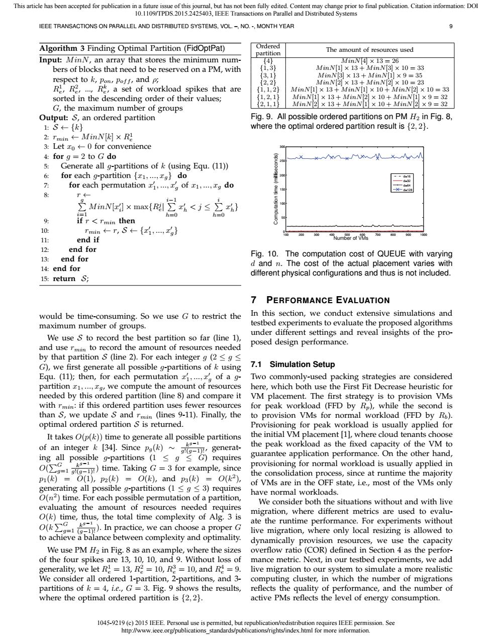
This article has been accepted for publication in a future issue of this journal,but has not been fully edited.Content may change prior to final publication.Citation information:DOI 10.1109/TPDS.2015.2425403,IEEE Transactions on Parallel and Distributed Systems IEEE TRANSACTIONS ON PARALLEL AND DISTRIBUTED SYSTEMS,VOL.-.NO.-,MONTH YEAR 9 Algorithm 3 Finding Optimal Partition(FidOptPat) Ordered partition The amount of resources used Input:MinN,an array that stores the minimum num- 47 MinW4×13=26 bers of blocks that need to be reserved on a PM,with {1,3} MinN[1]×13+MinN[3]×10=33 {3,1 respect to k,Pon,Poff,and p; MimN3×13+MimN[l]×9=35 {2,2} MinN[2×13+MinN[2]×10=23 R,R2,...,Re,a set of workload spikes that are 1.1,2 MinN[1]×13+MinN[1]×10+MinN2]×10=33 sorted in the descending order of their values; 1,2,1 MimN×13+MimN2×10+MinN[1]×9=32 G,the maximum number of groups 2,1,1 MinN[2×13+MimN[1]×10+MinN[2]×9=32 Output:S,an ordered partition Fig.9.All possible ordered partitions on PM H2 in Fig.8, 1:S←{} where the optimal ordered partition result is {2,2). 2:Tmin←MinN[内×Rg 3:Let zo 0 for convenience 4:for g=2 to G do 5: Generate all g-partitions of k(using Equ.(11)) for each g-partition [r1,...,g}do for each permutation z1,.,of 1,...,g do T← h=0 9: if r rmin then 10: Tmin←T,S←{i,,tg} 20的 80 90 11: end if Numb8rof微s 12: end for Fig.10.The computation cost of QUEUE with varying 13: end for d and n.The cost of the actual placement varies with 14:end for 15:return S; different physical configurations and thus is not included. 7 PERFORMANCE EVALUATION would be time-consuming.So we use G to restrict the In this section,we conduct extensive simulations and maximum number of groups. testbed experiments to evaluate the proposed algorithms We use S to record the best partition so far (line 1) under different settings and reveal insights of the pro- and use rmin to record the amount of resources needed posed design performance. by that partition S(line 2).For each integer g(2<g< G),we first generate all possible g-partitions of k using 7.1 Simulation Setup Equ.(11);then,for each permutation x1,...,of a g- Two commonly-used packing strategies are considered partition x1,...,g,we compute the amount of resources here,which both use the First Fit Decrease heuristic for needed by this ordered partition(line 8)and compare it VM placement.The first strategy is to provision VMs with rmin:if this ordered partition uses fewer resources for peak workload (FFD by Rp),while the second is than S,we update S and rmin (lines 9-11).Finally,the to provision VMs for normal workload (FFD by Ro). optimal ordered partition S is returned. Provisioning for peak workload is usually applied for It takes O(p())time to generate all possible partitions the initial VM placement [1],where cloud tenants choose k9-1 of an integer k [34].Since pa(k),generat- the peak workload as the fixed capacity of the VM to ing all possible g-partitions (1<gG)requires guarantee application performance.On the other hand, O)time.Taking G3 for example,since k9-1 provisioning for normal workload is usually applied in p1()=O(1),p2(k)=O(k),andp3(k)=O(k2), the consolidation process,since at runtime the majority of VMs are in the OFF state,i.e.,most of the VMs only generating all possible g-partitions(1<g 3)requires O(n2)time.For each possible permutation of a partition, have normal workloads. We consider both the situations without and with live evaluating the amount of resources needed requires migration,where different metrics are used to evalu- O(k)time,thus,the total time complexity of Alg.3 is ,k91 Ok∑g1合.In practice,wecan choosea properG ate the runtime performance.For experiments without live migration,where only local resizing is allowed to to achieve a balance between complexity and optimality. dynamically provision resources,we use the capacity We use PM H2 in Fig.8 as an example,where the sizes overflow ratio (COR)defined in Section 4 as the perfor- of the four spikes are 13,10,10,and 9.Without loss of mance metric.Next,in our testbed experiments,we add generality,we let RI=13,R2=10,R=10,and R=9.live migration to our system to simulate a more realistic We consider all ordered 1-partition,2-partitions,and 3- computing cluster,in which the number of migrations partitions of k=4,i.e.,G=3.Fig.9 shows the results,reflects the quality of performance,and the number of where the optimal ordered partition is [2,2). active PMs reflects the level of energy consumption. 1045-9219(c)2015 IEEE.Personal use is permitted,but republication/redistribution requires IEEE permission.See http://www.ieee.org/publications standards/publications/rights/index.html for more information.1045-9219 (c) 2015 IEEE. Personal use is permitted, but republication/redistribution requires IEEE permission. See http://www.ieee.org/publications_standards/publications/rights/index.html for more information. This article has been accepted for publication in a future issue of this journal, but has not been fully edited. Content may change prior to final publication. Citation information: DOI 10.1109/TPDS.2015.2425403, IEEE Transactions on Parallel and Distributed Systems IEEE TRANSACTIONS ON PARALLEL AND DISTRIBUTED SYSTEMS, VOL. –, NO. -, MONTH YEAR 9 Algorithm 3 Finding Optimal Partition (FidOptPat) Input: M inN, an array that stores the minimum num￾bers of blocks that need to be reserved on a PM, with respect to k, pon, poff , and ρ; R1 e , R2 e , ..., Rk e , a set of workload spikes that are sorted in the descending order of their values; G, the maximum number of groups Output: S, an ordered partition 1: S ← {k} 2: rmin ← M inN[k] × R1 e 3: Let x0 ← 0 for convenience 4: for g = 2 to G do 5: Generate all g-partitions of k (using Equ. (11)) 6: for each g-partition {x1, ..., xg} do 7: for each permutation x ′ 1 , ..., x′ g of x1, ..., xg do 8: r ← ∑g i=1 M inN[x ′ i ] × max{Rj e | i ∑−1 h=0 x ′ h < j ≤ ∑ i h=0 x ′ h } 9: if r < rmin then 10: rmin ← r, S ← {x ′ 1 , ..., x′ g} 11: end if 12: end for 13: end for 14: end for 15: return S; would be time-consuming. So we use G to restrict the maximum number of groups. We use S to record the best partition so far (line 1), and use rmin to record the amount of resources needed by that partition S (line 2). For each integer g (2 ≤ g ≤ G), we first generate all possible g-partitions of k using Equ. (11); then, for each permutation x ′ 1 , ..., x′ g of a g￾partition x1, ..., xg, we compute the amount of resources needed by this ordered partition (line 8) and compare it with rmin: if this ordered partition uses fewer resources than S, we update S and rmin (lines 9-11). Finally, the optimal ordered partition S is returned. It takes O(p(k)) time to generate all possible partitions of an integer k [34]. Since pg(k) ∼ k g−1 g!(g−1)! , generat￾ing all possible g-partitions (1 ≤ g ≤ G) requires O( ∑G g=1 k g−1 g!(g−1)!) time. Taking G = 3 for example, since p1(k) = O(1), p2(k) = O(k), and p3(k) = O(k 2 ), generating all possible g-partitions (1 ≤ g ≤ 3) requires O(n 2 ) time. For each possible permutation of a partition, evaluating the amount of resources needed requires O(k) time, thus, the total time complexity of Alg. 3 is O(k ∑G g=1 k g−1 (g−1)!). In practice, we can choose a proper G to achieve a balance between complexity and optimality. We use PM H2 in Fig. 8 as an example, where the sizes of the four spikes are 13, 10, 10, and 9. Without loss of generality, we let R1 e = 13, R2 e = 10, R3 e = 10, and R4 e = 9. We consider all ordered 1-partition, 2-partitions, and 3- partitions of k = 4, i.e., G = 3. Fig. 9 shows the results, where the optimal ordered partition is {2, 2}. Ordered The amount of resources used partition {4} M inN[4] × 13 = 26 {1, 3} M inN[1] × 13 + M inN[3] × 10 = 33 {3, 1} M inN[3] × 13 + M inN[1] × 9 = 35 {2, 2} M inN[2] × 13 + M inN[2] × 10 = 23 {1, 1, 2} M inN[1] × 13 + M inN[1] × 10 + M inN[2] × 10 = 33 {1, 2, 1} M inN[1] × 13 + M inN[2] × 10 + M inN[1] × 9 = 32 {2, 1, 1} M inN[2] × 13 + M inN[1] × 10 + M inN[2] × 9 = 32 Fig. 9. All possible ordered partitions on PM H2 in Fig. 8, where the optimal ordered partition result is {2, 2}. 100 200 300 400 500 600 700 800 900 1000 0 50 100 150 200 250 300 Number of VMs Computation time (milliseconds) d=16 d=32 d=64 d=128 Fig. 10. The computation cost of QUEUE with varying d and n. The cost of the actual placement varies with different physical configurations and thus is not included. 7 PERFORMANCE EVALUATION In this section, we conduct extensive simulations and testbed experiments to evaluate the proposed algorithms under different settings and reveal insights of the pro￾posed design performance. 7.1 Simulation Setup Two commonly-used packing strategies are considered here, which both use the First Fit Decrease heuristic for VM placement. The first strategy is to provision VMs for peak workload (FFD by Rp), while the second is to provision VMs for normal workload (FFD by Rb). Provisioning for peak workload is usually applied for the initial VM placement [1], where cloud tenants choose the peak workload as the fixed capacity of the VM to guarantee application performance. On the other hand, provisioning for normal workload is usually applied in the consolidation process, since at runtime the majority of VMs are in the OFF state, i.e., most of the VMs only have normal workloads. We consider both the situations without and with live migration, where different metrics are used to evalu￾ate the runtime performance. For experiments without live migration, where only local resizing is allowed to dynamically provision resources, we use the capacity overflow ratio (COR) defined in Section 4 as the perfor￾mance metric. Next, in our testbed experiments, we add live migration to our system to simulate a more realistic computing cluster, in which the number of migrations reflects the quality of performance, and the number of active PMs reflects the level of energy consumption