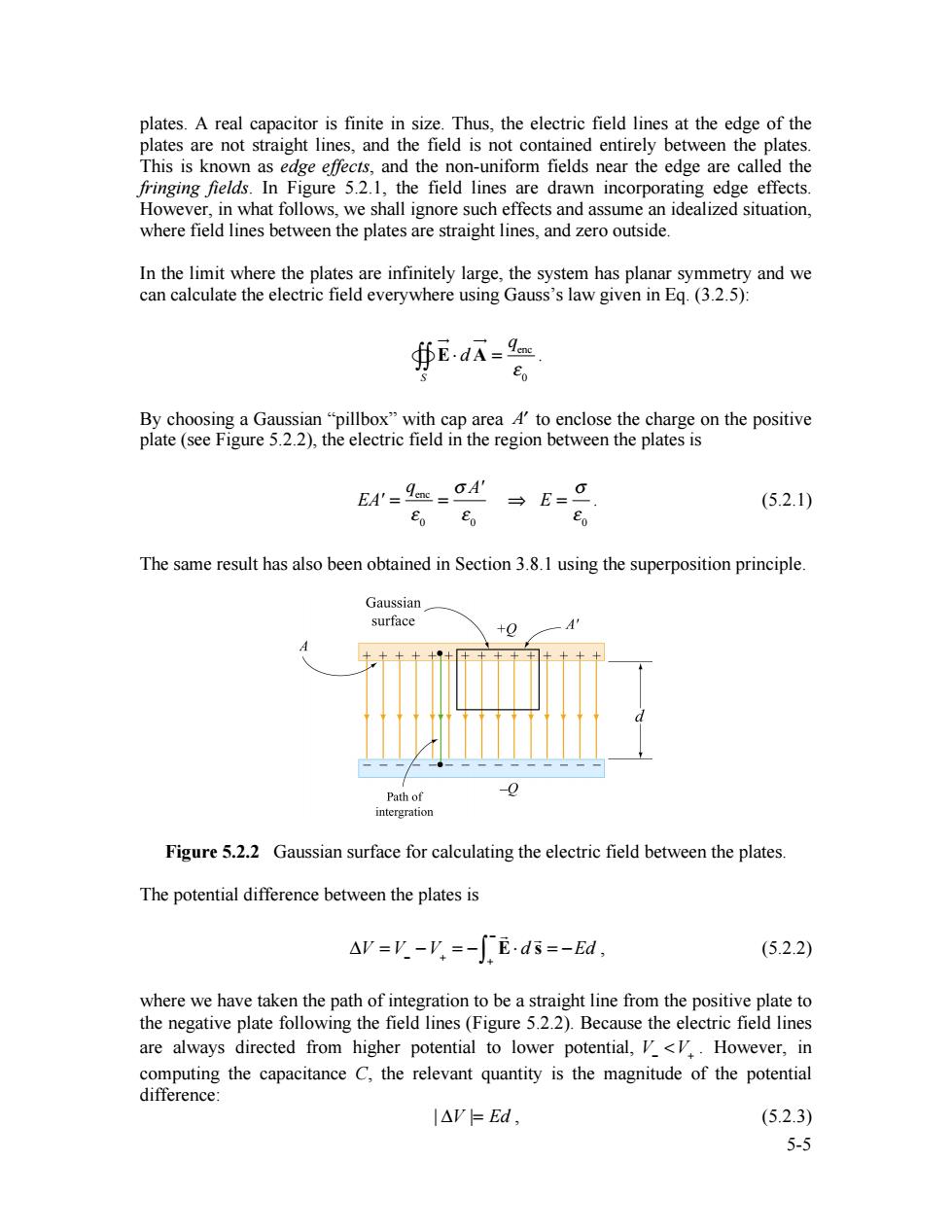
plates.A real capacitor is finite in size.Thus,the electric field lines at the edge of the plates are not straight lines,and the field is not contained entirely between the plates. This is known as edge effects,and the non-uniform fields near the edge are called the fringing fields.In Figure 5.2.1,the field lines are drawn incorporating edge effects However,in what follows,we shall ignore such effects and assume an idealized situation, where field lines between the plates are straight lines,and zero outside. In the limit where the plates are infinitely large,the system has planar symmetry and we can calculate the electric field everywhere using Gauss's law given in Eq.(3.2.5): ∯EdA=9 Eo By choosing a Gaussian "pillbox"with cap area A4'to enclose the charge on the positive plate (see Figure 5.2.2),the electric field in the region between the plates is EA'=9eE=A' (5.2.1) Eo →E= Eo The same result has also been obtained in Section 3.8.1 using the superposition principle. Gaussian surface +O -0 Path of intergration Figure 5.2.2 Gaussian surface for calculating the electric field between the plates. The potential difference between the plates is AV=V.-V,=-fE.ds=-Ed, (5.2.2) where we have taken the path of integration to be a straight line from the positive plate to the negative plate following the field lines(Figure 5.2.2).Because the electric field lines are always directed from higher potential to lower potential,V<V..However,in computing the capacitance C,the relevant quantity is the magnitude of the potential difference: l△V=Ed, (5.2.3) 5-55-5 plates. A real capacitor is finite in size. Thus, the electric field lines at the edge of the plates are not straight lines, and the field is not contained entirely between the plates. This is known as edge effects, and the non-uniform fields near the edge are called the fringing fields. In Figure 5.2.1, the field lines are drawn incorporating edge effects. However, in what follows, we shall ignore such effects and assume an idealized situation, where field lines between the plates are straight lines, and zero outside. In the limit where the plates are infinitely large, the system has planar symmetry and we can calculate the electric field everywhere using Gauss’s law given in Eq. (3.2.5): E !" ! d A !" S #"" = qenc # 0 . By choosing a Gaussian “pillbox” with cap area A! to enclose the charge on the positive plate (see Figure 5.2.2), the electric field in the region between the plates is EA' = qenc ! 0 = " A' ! 0 # E = " ! 0 . (5.2.1) The same result has also been obtained in Section 3.8.1 using the superposition principle. Figure 5.2.2 Gaussian surface for calculating the electric field between the plates. The potential difference between the plates is !V = V" "V+ = " ! E# d ! s + " $ = "Ed , (5.2.2) where we have taken the path of integration to be a straight line from the positive plate to the negative plate following the field lines (Figure 5.2.2). Because the electric field lines are always directed from higher potential to lower potential, V! <V+ . However, in computing the capacitance C, the relevant quantity is the magnitude of the potential difference: | !V |= Ed , (5.2.3)