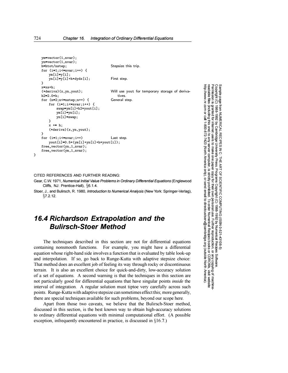
724 Chapter 16. Integration of Ordinary Differential Equations ym=vector(1,nvar): yn=vector(1,nvar); h=htot/nstep; Stepsize this trip for (i=1;i<-nvar;i++){ ym[i]=y[1]; yn[i]=y[i]+h*dydx [i]; First step. x=xs+h; (*derivs)(x,yn,yout); Will use yout for temporary storage of deriva- h2=2.0*h; tives. for (n=2;n<=nstep;n++){ General step. for (i=1;i<=nvar;i++){ swap=ym[i]+h2*yout [i]; ym[i]=yn[i]; 83g yn[i]=swap; 19881992 x+=h; 11800 NUMERICAL (*derivs)(x,yn,yout) } for (is1;i<=nvar;i++) Last step. yout [i]=0.5*(ym[i]+yn[i]+h*yout [i]); RECIPES free_vector(yn,1,nvar); free_vector(ym,1,nvar); 2 server computer, (North America to make one paper University Press. THE ART CITED REFERENCES AND FURTHER READING: Gear,C.W.1971,Numerical Initial Value Problems in Ordinary Differential Eguations(Englewood Programs Cliffs,NJ:Prentice-Hall).86.1.4. copy for their Stoer.J.,and Bulirsch.R.1980.Introduction to Numerical Analysis(New York:Springer-Verlag). S7.2.12. 16.4 Richardson Extrapolation and the 1881892 OF SCIENTIFIC COMPUTING(ISBN Bulirsch-Stoer Method e uurggoglrion Numerical 1021 The techniques described in this section are not for differential equations Recipes 43108 containing nonsmooth functions.For example,you might have a differential equation whose right-hand side involves a function that is evaluated by table look-up (outside and interpolation.If so,go back to Runge-Kutta with adaptive stepsize choice: That method does an excellent job of feeling its way through rocky or discontinuous North Software. terrain.It is also an excellent choice for quick-and-dirty,low-accuracy solution of a set of equations.A second warning is that the techniques in this section are not particularly good for differential equations that have singular points inside the interval of integration.A regular solution must tiptoe very carefully across such machine points.Runge-Kutta with adaptive stepsize can sometimes effect this;more generally, there are special techniques available for such problems,beyond our scope here. Apart from those two caveats,we believe that the Bulirsch-Stoer method, discussed in this section,is the best known way to obtain high-accuracy solutions to ordinary differential equations with minimal computational effort.(A possible exception,infrequently encountered in practice,is discussed in $16.7.)724 Chapter 16. Integration of Ordinary Differential Equations Permission is granted for internet users to make one paper copy for their own personal use. Further reproduction, or any copyin Copyright (C) 1988-1992 by Cambridge University Press. Programs Copyright (C) 1988-1992 by Numerical Recipes Software. Sample page from NUMERICAL RECIPES IN C: THE ART OF SCIENTIFIC COMPUTING (ISBN 0-521-43108-5) g of machine￾readable files (including this one) to any server computer, is strictly prohibited. To order Numerical Recipes books or CDROMs, visit website http://www.nr.com or call 1-800-872-7423 (North America only), or send email to directcustserv@cambridge.org (outside North America). ym=vector(1,nvar); yn=vector(1,nvar); h=htot/nstep; Stepsize this trip. for (i=1;i<=nvar;i++) { ym[i]=y[i]; yn[i]=y[i]+h*dydx[i]; First step. } x=xs+h; (*derivs)(x,yn,yout); Will use yout for temporary storage of deriva￾h2=2.0*h; tives. for (n=2;n<=nstep;n++) { General step. for (i=1;i<=nvar;i++) { swap=ym[i]+h2*yout[i]; ym[i]=yn[i]; yn[i]=swap; } x += h; (*derivs)(x,yn,yout); } for (i=1;i<=nvar;i++) Last step. yout[i]=0.5*(ym[i]+yn[i]+h*yout[i]); free_vector(yn,1,nvar); free_vector(ym,1,nvar); } CITED REFERENCES AND FURTHER READING: Gear, C.W. 1971, Numerical Initial Value Problems in Ordinary Differential Equations (Englewood Cliffs, NJ: Prentice-Hall), §6.1.4. Stoer, J., and Bulirsch, R. 1980, Introduction to Numerical Analysis (New York: Springer-Verlag), §7.2.12. 16.4 Richardson Extrapolation and the Bulirsch-Stoer Method The techniques described in this section are not for differential equations containing nonsmooth functions. For example, you might have a differential equation whose right-hand side involves a function that is evaluated by table look-up and interpolation. If so, go back to Runge-Kutta with adaptive stepsize choice: That method does an excellent job of feeling its way through rocky or discontinuous terrain. It is also an excellent choice for quick-and-dirty, low-accuracy solution of a set of equations. A second warning is that the techniques in this section are not particularly good for differential equations that have singular points inside the interval of integration. A regular solution must tiptoe very carefully across such points. Runge-Kutta with adaptive stepsize can sometimes effect this; more generally, there are special techniques available for such problems, beyond our scope here. Apart from those two caveats, we believe that the Bulirsch-Stoer method, discussed in this section, is the best known way to obtain high-accuracy solutions to ordinary differential equations with minimal computational effort. (A possible exception, infrequently encountered in practice, is discussed in §16.7.)