4 2 low redundancy high redundancy FIG.2 Simulated data of (x,y)for camera A.The signal and noise variances o landare graphically represented by the two FIG.3 A spectrum of possible redundancies in data from the two lines subtending the cloud of data.Note that the largest direction separate measurements rI and r2.The two measurements on the of variance does not lie along the basis of the recording (xA,yA)but left are uncorrelated because one can not predict one from the other rather along the best-fit line. Conversely,the two measurements on the right are highly correlated indicating highly redundant measurements can be extracted.There exists no absolute scale for noise but B.Redundancy rather all noise is quantified relative to the signal strength.A common measure is the signal-to-noise ratio (SNR),or a ratio of variances o-, Figure 2 hints at an additional confounding factor in our data -redundancy.This issue is particularly evident in the example of the spring.In this case multiple sensors record the same dynamic information.Reexamine Figure 2 and ask whether SNR= 6ig吧 it was really necessary to record 2 variables.Figure 3 might reflect a range of possibile plots between two arbitrary mea- surement types ri and r2.The left-hand panel depicts two A high SNR 1)indicates a high precision measurement, recordings with no apparent relationship.Because one can not while a low SNR indicates very noisy data. predict ri from r2,one says that ri and r2 are uncorrelated. Let's take a closer examination of the data from camera On the other extreme,the right-hand panel of Figure 3 de- A in Figure 2.Remembering that the spring travels in a picts highly correlated recordings.This extremity might be straight line,every individual camera should record motion in achieved by several means: a straight line as well.Therefore,any spread deviating from straight-line motion is noise.The variance due to the signal and noise are indicated by each line in the diagram.The ratio .A plot of (xA.xB)if cameras A and B are very nearby of the two lengths measures how skinny the cloud is:possibil- ities include a thin line (SNR>1),a circle (SNR =1)or even .A plot of (xA,)where x is in meters and fa is in worse.By positing reasonably good measurements,quantita- inches. tively we assume that directions with largest variances in our measurement space contain the dynamics of interest.In Fig- ure 2 the direction with the largest variance is notfa=(1,0) Clearly in the right panel of Figure 3 it would be more mean- nor y =(0,1),but the direction along the long axis of the ingful to just have recorded a single variable,not both.Why? cloud.Thus,by assumption the dynamics of interest exist Because one can calculate ri from r2 (or vice versa)using the along directions with largest variance and presumably high- best-fit line.Recording solely one response would express the est SNR data more concisely and reduce the number of sensor record- ings(2-1 variables).Indeed,this is the central idea behind Our assumption suggests that the basis for which we are dimensional reduction. searching is not the naive basis because these directions (i.e. (xA,yA))do not correspond to the directions of largest vari- ance.Maximizing the variance (and by assumption the SNR) corresponds to finding the appropriate rotation of the naive C.Covariance Matrix basis.This intuition corresponds to finding the direction indi- cated by the line in Figure 2.In the 2-dimensional case of Figure 2 the direction of largest variance corresponds to the In a 2 variable case it is simple to identify redundant cases by best-fit line for the data cloud.Thus,rotating the naive basis finding the slope of the best-fit line and judging the quality of to lie parallel to the best-fit line would reveal the direction of the fit.How do we quantify and generalize these notions to motion of the spring for the 2-D case.How do we generalize arbitrarily higher dimensions?Consider two sets of measure- this notion to an arbitrary number of dimensions?Before we ments with zero means approach this question we need to examine this issue from a second perspective. A={a1,a2,,an},B={b1,b2,,bn}4 σ 2 signal σ 2 noise x y FIG. 2 Simulated data of (x,y) for camera A. The signal and noise variances σ 2 signal and σ 2 noise are graphically represented by the two lines subtending the cloud of data. Note that the largest direction of variance does not lie along the basis of the recording (xA,yA) but rather along the best-fit line. can be extracted. There exists no absolute scale for noise but rather all noise is quantified relative to the signal strength. A common measure is the signal-to-noise ratio (SNR), or a ratio of variances σ 2 , SNR = σ 2 signal σ 2 noise . A high SNR ( 1) indicates a high precision measurement, while a low SNR indicates very noisy data. Let’s take a closer examination of the data from camera A in Figure 2. Remembering that the spring travels in a straight line, every individual camera should record motion in a straight line as well. Therefore, any spread deviating from straight-line motion is noise. The variance due to the signal and noise are indicated by each line in the diagram. 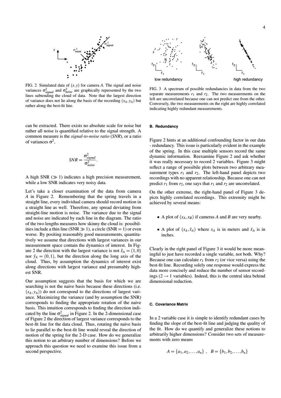The ratio of the two lengths measures how skinny the cloud is: possibil￾ities include a thin line (SNR  1), a circle (SNR = 1) or even worse. By positing reasonably good measurements, quantita￾tively we assume that directions with largest variances in our measurement space contain the dynamics of interest. In Fig￾ure 2 the direction with the largest variance is not ˆxA = (1,0) nor ˆyA = (0,1), but the direction along the long axis of the cloud. Thus, by assumption the dynamics of interest exist along directions with largest variance and presumably high￾est SNR. Our assumption suggests that the basis for which we are searching is not the naive basis because these directions (i.e. (xA,yA)) do not correspond to the directions of largest vari￾ance. Maximizing the variance (and by assumption the SNR) corresponds to finding the appropriate rotation of the naive basis. This intuition corresponds to finding the direction indi￾cated by the line σ 2 signal in Figure 2. In the 2-dimensional case of Figure 2 the direction of largest variance corresponds to the best-fit line for the data cloud. Thus, rotating the naive basis to lie parallel to the best-fit line would reveal the direction of motion of the spring for the 2-D case. How do we generalize this notion to an arbitrary number of dimensions? Before we approach this question we need to examine this issue from a second perspective. low redundancy high redundancy r 1 r 2 r 1 r 2 r 1 r 2 FIG. 3 A spectrum of possible redundancies in data from the two separate measurements r1 and r2. The two measurements on the left are uncorrelated because one can not predict one from the other. Conversely, the two measurements on the right are highly correlated indicating highly redundant measurements. B. Redundancy Figure 2 hints at an additional confounding factor in our data - redundancy. This issue is particularly evident in the example of the spring. In this case multiple sensors record the same dynamic information. Reexamine Figure 2 and ask whether it was really necessary to record 2 variables. Figure 3 might reflect a range of possibile plots between two arbitrary mea￾surement types r1 and r2. The left-hand panel depicts two recordings with no apparent relationship. Because one can not predict r1 from r2, one says that r1 and r2 are uncorrelated. On the other extreme, the right-hand panel of Figure 3 de￾picts highly correlated recordings. This extremity might be achieved by several means: • A plot of (xA,xB) if cameras A and B are very nearby. • A plot of (xA,x˜A) where xA is in meters and ˜xA is in inches. Clearly in the right panel of Figure 3 it would be more mean￾ingful to just have recorded a single variable, not both. Why? Because one can calculate r1 from r2 (or vice versa) using the best-fit line. Recording solely one response would express the data more concisely and reduce the number of sensor record￾ings (2 → 1 variables). Indeed, this is the central idea behind dimensional reduction. C. Covariance Matrix In a 2 variable case it is simple to identify redundant cases by finding the slope of the best-fit line and judging the quality of the fit. How do we quantify and generalize these notions to arbitrarily higher dimensions? Consider two sets of measure￾ments with zero means A = {a1,a2,...,an} , B = {b1,b2,...,bn}