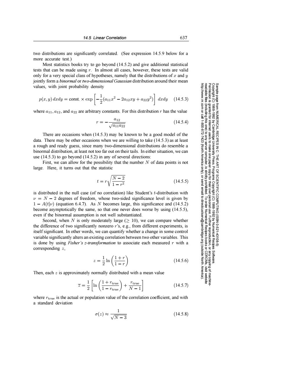
14.5 Linear Correlation 637 two distributions are significantly correlated.(See expression 14.5.9 below for a more accurate test. Most statistics books try to go beyond (14.5.2)and give additional statistical tests that can be made using r.In almost all cases,however,these tests are valid only for a very special class of hypotheses,namely that the distributions of and y jointly form a binormal or two-dimensional Gaussian distribution around their mean values,with joint probability density p(x,y)dxdy const.x exp a2-2aw+a） dxdy (14.5.3) 81 where a1,a12,and a22 are arbitrary constants.For this distribution r has the value 012 T三 (14.5.4) /a11a22 ICAL There are occasions when(14.5.3)may be known to be a good model of the data.There may be other occasions when we are willing to take(14.5.3)as at least a rough and ready guess,since many two-dimensional distributions do resemble a binormal distribution,at least not too far out on their tails.In either situation,we can use (14.5.3)to go beyond(14.5.2)in any of several directions: First,we can allow for the possibility that the number N of data points is not 曼芸2物09州 large.Here,it turns out that the statistic N-2 t=1 量色鸟6 V1-2 (14.5.5) is distributed in the null case (of no correlation)like Student's t-distribution with =N-2 degrees of freedom,whose two-sided significance level is given by 6 1-A(t)(equation 6.4.7).As N becomes large,this significance and (14.5.2) become asymptotically the same,so that one never does worse by using(14.5.5), even if the binormal assumption is not well substantiated. Second,when N is only moderately large (>10),we can compare whether the difference of two significantly nonzero r's,e.g.,from different experiments,is itself significant.In other words,we can quantify whether a change in some control Numerica 10621 variable significantly alters an existing correlation between two other variables.This 43106 is done by using Fisher's z-transformation to associate each measured r with a corresponding 2, a=() (14.5.6) Then,each z is approximately normally distributed with a mean value 1 (1+Ttrue 2(-re +N一 Ttrue (14.5.7) where rtrue is the actual or population value of the correlation coefficient,and with a standard deviation .1 ()≈√N-3 (14.5.8)14.5 Linear Correlation 637 Permission is granted for internet users to make one paper copy for their own personal use. Further reproduction, or any copyin Copyright (C) 1988-1992 by Cambridge University Press. Programs Copyright (C) 1988-1992 by Numerical Recipes Software. Sample page from NUMERICAL RECIPES IN C: THE ART OF SCIENTIFIC COMPUTING (ISBN 0-521-43108-5) g of machine￾readable files (including this one) to any server computer, is strictly prohibited. To order Numerical Recipes books or CDROMs, visit website http://www.nr.com or call 1-800-872-7423 (North America only), or send email to directcustserv@cambridge.org (outside North America). two distributions are significantly correlated. (See expression 14.5.9 below for a more accurate test.) Most statistics books try to go beyond (14.5.2) and give additional statistical tests that can be made using r. In almost all cases, however, these tests are valid only for a very special class of hypotheses, namely that the distributions of x and y jointly form a binormal or two-dimensional Gaussian distribution around their mean values, with joint probability density p(x, y) dxdy = const. × exp  −1 2 (a11x2 − 2a12xy + a22y2)  dxdy (14.5.3) where a11, a12, and a22 are arbitrary constants. For this distribution r has the value r = − a12 √a11a22 (14.5.4) There are occasions when (14.5.3) may be known to be a good model of the data. There may be other occasions when we are willing to take (14.5.3) as at least a rough and ready guess, since many two-dimensional distributions do resemble a binormal distribution, at least not too far out on their tails. In either situation, we can use (14.5.3) to go beyond (14.5.2) in any of several directions: First, we can allow for the possibility that the number N of data points is not large. Here, it turns out that the statistic t = r N − 2 1 − r2 (14.5.5) is distributed in the null case (of no correlation) like Student’s t-distribution with ν = N − 2 degrees of freedom, whose two-sided significance level is given by 1 − A(t|ν) (equation 6.4.7). As N becomes large, this significance and (14.5.2) become asymptotically the same, so that one never does worse by using (14.5.5), even if the binormal assumption is not well substantiated. Second, when N is only moderately large (≥ 10), we can compare whether the difference of two significantly nonzero r’s, e.g., from different experiments, is itself significant. In other words, we can quantify whether a change in some control variable significantly alters an existing correlation between two other variables. This is done by using Fisher’s z-transformation to associate each measured r with a corresponding z, z = 1 2 ln 1 + r 1 − r  (14.5.6) Then, each z is approximately normally distributed with a mean value z = 1 2  ln 1 + rtrue 1 − rtrue  + rtrue N − 1  (14.5.7) where rtrue is the actual or population value of the correlation coefficient, and with a standard deviation σ(z) ≈ 1 √N − 3 (14.5.8)