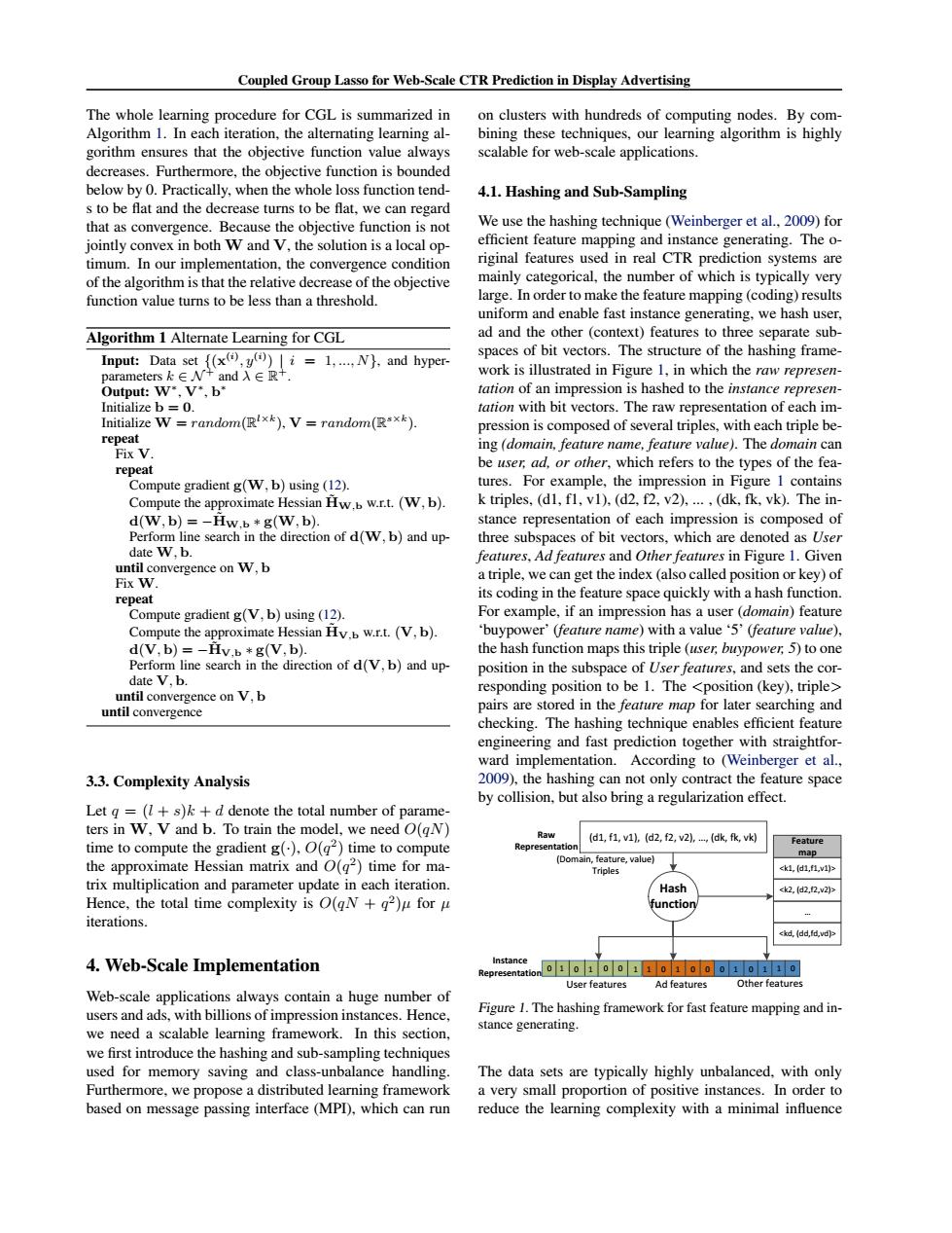
Coupled Group Lasso for Web-Scale CTR Prediction in Display Advertising The whole learning procedure for CGL is summarized in on clusters with hundreds of computing nodes.By com- Algorithm 1.In each iteration,the alternating learning al- bining these techniques,our learning algorithm is highly gorithm ensures that the objective function value always scalable for web-scale applications. decreases.Furthermore,the objective function is bounded below by 0.Practically.when the whole loss function tend- 4.1.Hashing and Sub-Sampling s to be flat and the decrease turns to be flat,we can regard that as convergence.Because the objective function is not We use the hashing technique(Weinberger et al.,2009)for jointly convex in both W and V,the solution is a local op- efficient feature mapping and instance generating.The o- timum.In our implementation,the convergence condition riginal features used in real CTR prediction systems are of the algorithm is that the relative decrease of the objective mainly categorical,the number of which is typically very function value turns to be less than a threshold. large.In order to make the feature mapping(coding)results uniform and enable fast instance generating,we hash user, Algorithm 1 Alternate Learning for CGL ad and the other(context)features to three separate sub- Input:Data set {(x(,()i=1,...N),and hyper- spaces of bit vectors.The structure of the hashing frame- parameters k∈W+and入∈R+ work is illustrated in Figure 1,in which the raw represen- Output:W*.V*.b* tation of an impression is hashed to the instance represen- Initialize b=0. tation with bit vectors.The raw representation of each im- Initialize W=random(R!xk),V=random(*xk) pression is composed of several triples,with each triple be- repeat Fix V ing(domain,feature name,feature value).The domain can repeat be user,ad,or other,which refers to the types of the fea- Compute gradient g(W,b)using (12). tures.For example,the impression in Figure 1 contains Compute the approximate Hessian Hw.b w.r.t.(W,b). k triples,(d1,fl,v1),(d2,f2,v2),...,(dk,fk,vk).The in- d(W,b)=-Hw.b*g(W,b). stance representation of each impression is composed of Perform line search in the direction of d(W,b)and up- three subspaces of bit vectors,which are denoted as User date W.b. features,Ad features and Other features in Figure 1.Given until convergence on W,b a triple,we can get the index (also called position or key)of Fix W. repeat its coding in the feature space quickly with a hash function. Compute gradient g(V,b)using(12). For example,if an impression has a user(domain)feature Compute the approximate Hessian Hv.b w.r.t.(V,b). buypower'(feature name)with a value'5'(feature value), d(V,b)=-Hv.b *g(V,b). the hash function maps this triple (user,buypower,5)to one Perform line search in the direction of d(V,b)and up- position in the subspace of User features,and sets the cor- date V.b. responding position to be 1.The <position(key),triple> until convergence on V,b until convergence pairs are stored in the feature map for later searching and checking.The hashing technique enables efficient feature engineering and fast prediction together with straightfor- ward implementation.According to (Weinberger et al., 3.3.Complexity Analysis 2009),the hashing can not only contract the feature space by collision,but also bring a regularization effect. Let g =(7+s)k +d denote the total number of parame- ters in W,V and b.To train the model,we need O(qN) (d1,f1,v1,(d2,f2,v2,,(dk,fkk time to compute the gradient g(),O(g2)time to compute Feature epresentation map the approximate Hessian matrix and O(q2)time for ma- (Domain,feature,value) Triples <k1d1.1v1> trix multiplication and parameter update in each iteration. Hash <k2d2,2,v2> Hence,the total time complexity is O(gN +2)u for u function iterations kd,(dd,fd.vd)> 4.Web-Scale Implementation Instance Representation o 1 0 1 00 1 1 0 1 00 0 1 0 11 0 User features Ad features Other features Web-scale applications always contain a huge number of users and ads,with billions of impression instances.Hence, Figure 1.The hashing framework for fast feature mapping and in- we need a scalable learning framework.In this section, stance generating. we first introduce the hashing and sub-sampling techniques used for memory saving and class-unbalance handling. The data sets are typically highly unbalanced,with only Furthermore,we propose a distributed learning framework a very small proportion of positive instances.In order to based on message passing interface(MPD),which can run reduce the learning complexity with a minimal influenceCoupled Group Lasso for Web-Scale CTR Prediction in Display Advertising The whole learning procedure for CGL is summarized in Algorithm 1. In each iteration, the alternating learning al￾gorithm ensures that the objective function value always decreases. Furthermore, the objective function is bounded below by 0. Practically, when the whole loss function tend￾s to be flat and the decrease turns to be flat, we can regard that as convergence. Because the objective function is not jointly convex in both W and V, the solution is a local op￾timum. In our implementation, the convergence condition of the algorithm is that the relative decrease of the objective function value turns to be less than a threshold. Algorithm 1 Alternate Learning for CGL Input: Data set {(x (i) , y(i) ) | i = 1, ..., N}, and hyper￾parameters k ∈ N + and λ ∈ R +. Output: W∗ , V∗ , b ∗ Initialize b = 0. Initialize W = random(R l×k ), V = random(R s×k ). repeat Fix V. repeat Compute gradient g(W, b) using (12). Compute the approximate Hessian H˜ W,b w.r.t. (W, b). d(W, b) = −H˜ W,b ∗ g(W, b). Perform line search in the direction of d(W, b) and up￾date W, b. until convergence on W, b Fix W. repeat Compute gradient g(V, b) using (12). Compute the approximate Hessian H˜ V,b w.r.t. (V, b). d(V, b) = −H˜ V,b ∗ g(V, b). Perform line search in the direction of d(V, b) and up￾date V, b. until convergence on V, b until convergence 3.3. Complexity Analysis Let q = (l + s)k + d denote the total number of parame￾ters in W, V and b. To train the model, we need O(qN) time to compute the gradient g(·), O(q 2 ) time to compute the approximate Hessian matrix and O(q 2 ) time for ma￾trix multiplication and parameter update in each iteration. Hence, the total time complexity is O(qN + q 2 )µ for µ iterations. 4. Web-Scale Implementation Web-scale applications always contain a huge number of users and ads, with billions of impression instances. Hence, we need a scalable learning framework. In this section, we first introduce the hashing and sub-sampling techniques used for memory saving and class-unbalance handling. Furthermore, we propose a distributed learning framework based on message passing interface (MPI), which can run on clusters with hundreds of computing nodes. By com￾bining these techniques, our learning algorithm is highly scalable for web-scale applications. 4.1. Hashing and Sub-Sampling We use the hashing technique (Weinberger et al., 2009) for efficient feature mapping and instance generating. The o￾riginal features used in real CTR prediction systems are mainly categorical, the number of which is typically very large. In order to make the feature mapping (coding) results uniform and enable fast instance generating, we hash user, ad and the other (context) features to three separate sub￾spaces of bit vectors. The structure of the hashing frame￾work is illustrated in Figure 1, in which the raw represen￾tation of an impression is hashed to the instance represen￾tation with bit vectors. The raw representation of each im￾pression is composed of several triples, with each triple be￾ing (domain, feature name, feature value). The domain can be user, ad, or other, which refers to the types of the fea￾tures. For example, the impression in Figure 1 contains k triples, (d1, f1, v1), (d2, f2, v2), ... , (dk, fk, vk). The in￾stance representation of each impression is composed of three subspaces of bit vectors, which are denoted as User features, Ad features and Other features in Figure 1. Given a triple, we can get the index (also called position or key) of its coding in the feature space quickly with a hash function. For example, if an impression has a user (domain) feature ‘buypower’ (feature name) with a value ‘5’ (feature value), the hash function maps this triple (user, buypower, 5) to one position in the subspace of User features, and sets the cor￾responding position to be 1. The <position (key), triple> pairs are stored in the feature map for later searching and checking. The hashing technique enables efficient feature engineering and fast prediction together with straightfor￾ward implementation. According to (Weinberger et al., 2009), the hashing can not only contract the feature space by collision, but also bring a regularization effect. Ad features Hash function Other features (d1, f1, v1), (d2, f2, v2), …, (dk, fk, vk) (Domain, feature, value) Triples <k1, (d1,f1,v1)> <k2, (d2,f2,v2)> … <kd, (dd,fd,vd)> Feature map Raw Representation Instance Representation User features 0 1 0 1 0 0 1 1 0 1 0 0 0 1 0 1 1 0 Figure 1. The hashing framework for fast feature mapping and in￾stance generating. The data sets are typically highly unbalanced, with only a very small proportion of positive instances. In order to reduce the learning complexity with a minimal influence