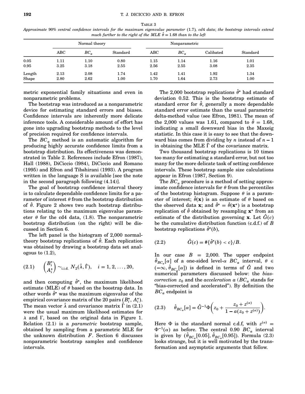
192 T.J.DICICCIO AND B.EFRON TABLE 3 Approximate 90%central confidence intervals for the maximum eigenvalue parameter (1.7).cd4 data:the bootstrap intervals extend much further to the right of the MLE=1.68 than to the left Normal theory Nonparametric ABC BCa Standard ABC BCa Calibated Standard 0.05 1.11 1.10 0.80 1.15 1.14 1.16 1.01 0.95 3.25 3.18 2.55 2.56 2.55 3.08 2.35 Length 2.13 2.08 1.74 1.42 1.41 1.92 1.34 Shape 2.80 2.62 1.00 1.70 1.64 2.73 1.00 metric exponential family situations and even in The 2,000 bootstrap replications had standard nonparametric problems. deviation 0.52.This is the bootstrap estimate of The bootstrap was introduced as a nonparametric standard error for 6,generally a more dependable device for estimating standard errors and biases. standard error estimate than the usual parametric Confidence intervals are inherently more delicate delta-method value (see Efron,1981).The mean of inference tools.A considerable amount of effort has the 2,000 values was 1.61,compared to =1.68, gone into upgrading bootstrap methods to the level indicating a small downward bias in the Maxeig of precision required for confidence intervals. statistic.In this case it is easy to see that the down- The BC method is an automatic algorithm for ward bias comes from dividing by n instead of n-1 producing highly accurate confidence limits from a in obtaining the MLE I of the covariance matrix. bootstrap distribution.Its effectiveness was demon- Two thousand bootstrap replications is 10 times strated in Table 2.References include Efron(1987), too many for estimating a standard error,but not too Hall (1988),DiCiccio (1984),DiCiccio and Romano many for the more delicate task of setting confidence (1995)and Efron and Tibshirani(1993).A program intervals.These bootstrap sample size calculations written in the language S is available [see the note appear in Efron(1987,Section 9). in the second paragraph following (4.14)]. The BC procedure is a method of setting approx- The goal of bootstrap confidence interval theory imate confidence intervals for 6 from the percentiles is to calculate dependable confidence limits for a pa- of the bootstrap histogram.Suppose e is a param- rameter of interest 6 from the bootstrap distribution eter of interest;0(x)is an estimate of based on of 6.Figure 2 shows two such bootstrap distribu- the observed data x;and*=(x*)is a bootstrap tions relating to the maximum eigenvalue param- replication of 6 obtained by resampling x*from an eter 0 for the cd4 data,(1.8).The nonparametric estimate of the distribution governing x.Let G(c) bootstrap distribution (on the right)will be dis- be the cumulative distribution function(c.d.f.)of B cussed in Section 6. bootstrap replications *(b), The left panel is the histogram of 2,000 normal- theory bootstrap replications of 6.Each replication (2.2) G(c)=#{(b)<c}/B was obtained by drawing a bootstrap data set anal- ogous to(1.2)】 In our case B =2,000.The upper endpoint Oc.[a]of a one-sided level-a BCa interval,0 2.1 iid.N2(,),i=1,2,..,20, (-OBc [a])is defined in terms of G and two numerical parameters discussed below:the bias. and then computing the maximum likelihood correction zo and the acceleration a(BCa stands for estimate (MLE)of based on the boostrap data.In "bias-corrected and accelerated").By definition the other words6*was the maximum eigenvalue of the BCa endpoint is empirical covariance matrix of the 20 pairs(B:,A). The mean vector A and covariance matrix I'in(2.1) (2.3) 20+2a) were the usual maximum likelihood estimates for c.al=G-1(2o+1-a(0+z@可 入and「，based on the original data in Figure 1. Relation (2.1)is a parametric bootstrap sample, Here d is the standard normal c.d.f,with z()= obtained by sampling from a parametric MLE for (a)as before.The central 0.90 BC interval the unknown distribution F.Section 6 discusses is given by (BC.[0.05],0BC.[0.95]).Formula (2.3) nonparametric bootstrap samples and confidence looks strange,but it is well motivated by the trans- intervals. formation and asymptotic arguments that follow.192 T. J. DICICCIO AND B. EFRON Table 3 Approximate 90% central confidence intervals for the maximum eigenvalue parameter 1:7‘, cd4 data; the bootstrap intervals extend much further to the right of the MLE θˆ = 1:68 than to the left Normal theory Nonparametric ABC BCa Standard ABC BCa Calibated Standard 0.05 1.11 1.10 0.80 1.15 1.14 1.16 1.01 0.95 3.25 3.18 2.55 2.56 2.55 3.08 2.35 Length 2.13 2.08 1.74 1.42 1.41 1.92 1.34 Shape 2.80 2.62 1.00 1.70 1.64 2.73 1.00 metric exponential family situations and even in nonparametric problems. The bootstrap was introduced as a nonparametric device for estimating standard errors and biases. Confidence intervals are inherently more delicate inference tools. A considerable amount of effort has gone into upgrading bootstrap methods to the level of precision required for confidence intervals. The BCa method is an automatic algorithm for producing highly accurate confidence limits from a bootstrap distribution. Its effectiveness was demon￾strated in Table 2. References include Efron (1987), Hall (1988), DiCiccio (l984), DiCiccio and Romano (1995) and Efron and Tibshirani (1993). A program written in the language S is available [see the note in the second paragraph following (4.14)]. The goal of bootstrap confidence interval theory is to calculate dependable confidence limits for a pa￾rameter of interest θ from the bootstrap distribution of θˆ. Figure 2 shows two such bootstrap distribu￾tions relating to the maximum eigenvalue param￾eter θ for the cd4 data, (1.8). The nonparametric bootstrap distribution (on the right) will be dis￾cussed in Section 6. The left panel is the histogram of 2,000 normal￾theory bootstrap replications of θˆ. Each replication was obtained by drawing a bootstrap data set anal￾ogous to (1.2), 2:1‘  B∗ i A∗ i  ∼i:i:d: N2 λˆ; 0ˆ ‘; i = 1; 2;: : :; 20; and then computing θˆ ∗ , the maximum likelihood estimate (MLE) of θ based on the boostrap data. In other words θˆ ∗ was the maximum eigenvalue of the empirical covariance matrix of the 20 pairs B∗ i ; A∗ i ‘. The mean vector λˆ and covariance matrix 0ˆ in (2.1) were the usual maximum likelihood estimates for λ and 0, based on the original data in Figure 1. Relation (2.1) is a parametric bootstrap sample, obtained by sampling from a parametric MLE for the unknown distribution F. Section 6 discusses nonparametric bootstrap samples and confidence intervals. The 2,000 bootstrap replications θˆ ∗ had standard deviation 0.52. This is the bootstrap estimate of standard error for θˆ, generally a more dependable standard error estimate than the usual parametric delta-method value (see Efron, 1981). The mean of the 2,000 values was 1.61, compared to θˆ = 1:68, indicating a small downward bias in the Maxeig statistic. In this case it is easy to see that the down￾ward bias comes from dividing by n instead of n − 1 in obtaining the MLE 0ˆ of the covariance matrix. Two thousand bootstrap replications is 10 times too many for estimating a standard error, but not too many for the more delicate task of setting confidence intervals. These bootstrap sample size calculations appear in Efron (1987, Section 9). The BCa procedure is a method of setting approx￾imate confidence intervals for θ from the percentiles of the bootstrap histogram. Suppose θ is a param￾eter of interest; θˆx‘ is an estimate of θ based on the observed data x; and θˆ ∗ = θˆx ∗ ‘ is a bootstrap replication of θˆ obtained by resampling x ∗ from an estimate of the distribution governing x. Let Gˆ c‘ be the cumulative distribution function (c.d.f.) of B bootstrap replications θˆ ∗ b‘, 2:2‘ Gˆ c‘ = #θˆ ∗ b‘ < c•/B: In our case B = 2,000. The upper endpoint θˆBCa ’α of a one-sided level-α BCa interval, θ ∈ −∞; θˆBCa ’α‘ is defined in terms of Gˆ and two numerical parameters discussed below: the bias￾correction z0 and the acceleration a (BCa stands for “bias-corrected and accelerated”). By definition the BCa endpoint is 2:3‘ θˆBCa ’α = Gˆ −18  z0 + z0 + z α‘ 1 − az0 + z α‘‘  : Here 8 is the standard normal c.d.f, with z α‘ = 8−1 α‘ as before. The central 0.90 BCa interval is given by θˆBCa ’0:05; θˆBCa ’0:95‘. Formula (2.3) looks strange, but it is well motivated by the trans￾formation and asymptotic arguments that follow.