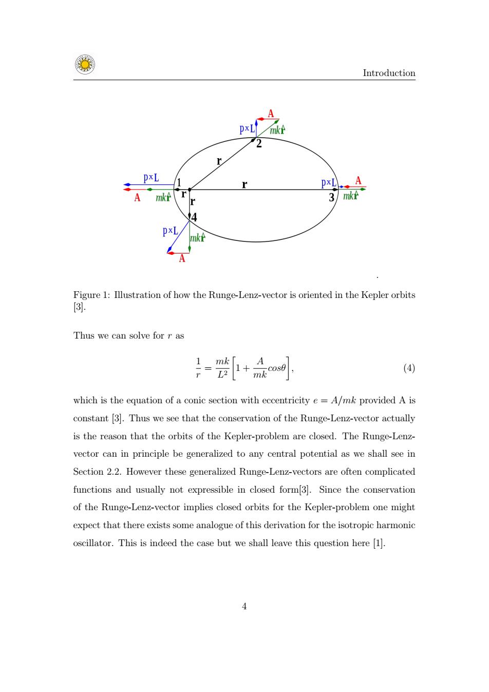
Introduction A pxL mkt pxL 1 A mkf 37 城≥ 4 Figure 1:Illustration of how the Runge-Lenz-vector is oriented in the Kepler orbits [3. Thus we can solve for r as mk (④) which is the equation of a conic section with eccentricity e=A/mk provided A is constant [3].Thus we see that the conservation of the Runge-Lenz-vector actually is the reason that the orbits of the Kepler-problem are closed.The Runge-Lenz- vector can in principle be generalized to any central potential as we shall see in Section 2.2.However these generalized Runge-Lenz-vectors are often complicated functions and usually not expressible in closed form[3].Since the conservation of the Runge-Lenz-vector implies closed orbits for the Kepler-problem one might expect that there exists some analogue of this derivation for the isotropic harmonic oscillator.This is indeed the case but we shall leave this question here [1]. 4Introduction . Figure 1: Illustration of how the Runge-Lenz-vector is oriented in the Kepler orbits [3]. Thus we can solve for r as 1 r = mk L2  1 + A mk cosθ , (4) which is the equation of a conic section with eccentricity e = A/mk provided A is constant [3]. Thus we see that the conservation of the Runge-Lenz-vector actually is the reason that the orbits of the Kepler-problem are closed. The Runge-Lenz￾vector can in principle be generalized to any central potential as we shall see in Section 2.2. However these generalized Runge-Lenz-vectors are often complicated functions and usually not expressible in closed form[3]. Since the conservation of the Runge-Lenz-vector implies closed orbits for the Kepler-problem one might expect that there exists some analogue of this derivation for the isotropic harmonic oscillator. This is indeed the case but we shall leave this question here [1]. 4