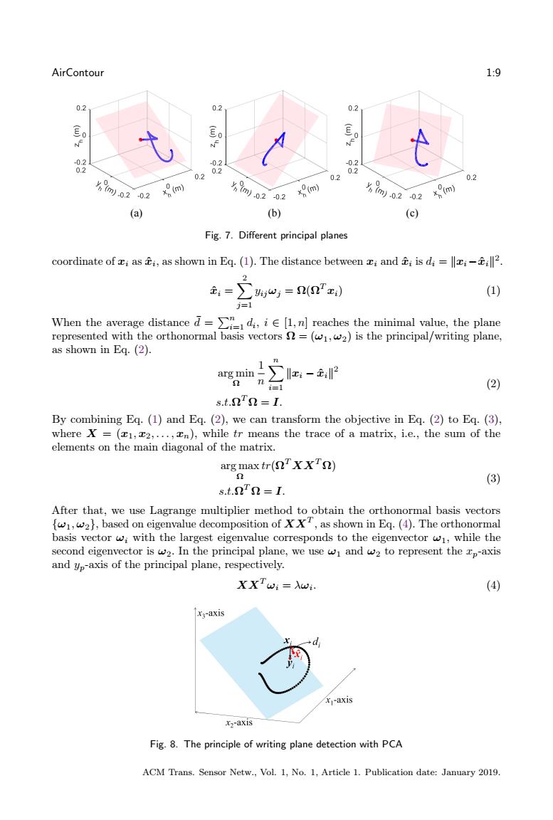
AirContour 1:9 0.2 0.2 0.2 Eo 83 0,2 0.2 83 0.2 02 0.2 m0202 m m)0202 x(m) %}m0202 m (a) (b) (c) Fig.7.Different principal planes coordinate of ci as ti,as shown in Eq.(1).The distance between xi and ti is di=xiil2. ,=∑%=n(n) (1) j=1 When the average distance-∑”_，d,i∈[l,nreaches the minimal value,the plane represented with the orthonormal basis vectors =(w,w2)is the principal/writing plane, as shown in Eq.(2). 11 arg min∑z:-主，2 =1 (2) s.t.nTn=I. By combining Eq.(1)and Eq.(2),we can transform the objective in Eq.(2)to Eq.(3), where X =(x1,x2,...,xn),while tr means the trace of a matrix,i.e.,the sum of the elements on the main diagonal of the matrix. arg max tr(nTXXTn) (3) s.t.nn=I. After that,we use Lagrange multiplier method to obtain the orthonormal basis vectors ,w2,based on eigenvalue decomposition ofT,as shown in Eq.(4).The orthonormal basis vector wi with the largest eigenvalue corresponds to the eigenvector w1,while the second eigenvector is w2.In the principal plane,we use wi and w2 to represent the p-axis and yp-axis of the principal plane,respectively. XXTwi=Xwi. (4) X;-axis x-axis x2-axis Fig.8.The principle of writing plane detection with PCA ACM Trans.Sensor Netw.,Vol.1,No.1,Article 1.Publication date:January 2019.AirContour 1:9 T3, x=55, y=25, [-0.18 0.18] T4, x=40, y=25, z=90, [-0.18 0.18], y取反-Right T5, z=50, y=20, [-0.18 0.18] (a) (b) (c) Fig. 7. Different principal planes coordinate of 𝑥𝑖 as 𝑥^𝑖 , as shown in Eq. (1). The distance between 𝑥𝑖 and 𝑥^𝑖 is 𝑑𝑖 = ‖𝑥𝑖−𝑥^𝑖‖ 2 . 𝑥^𝑖 = ∑︁ 2 𝑗=1 𝑦𝑖𝑗𝜔𝑗 = Ω(Ω 𝑇 𝑥𝑖) (1) When the average distance ¯𝑑 = ∑︀𝑛 𝑖=1 𝑑𝑖 , 𝑖 ∈ [1, 𝑛] reaches the minimal value, the plane represented with the orthonormal basis vectors Ω = (𝜔1, 𝜔2) is the principal/writing plane, as shown in Eq. (2). arg min Ω 1 𝑛 ∑︁𝑛 𝑖=1 ‖𝑥𝑖 − 𝑥^𝑖‖ 2 𝑠.𝑡.Ω 𝑇 Ω = 𝐼. (2) By combining Eq. (1) and Eq. (2), we can transform the objective in Eq. (2) to Eq. (3), where 𝑋 = (𝑥1, 𝑥2, . . . , 𝑥𝑛), while 𝑡𝑟 means the trace of a matrix, i.e., the sum of the elements on the main diagonal of the matrix. arg max Ω 𝑡𝑟(Ω 𝑇 𝑋𝑋𝑇 Ω) 𝑠.𝑡.Ω 𝑇 Ω = 𝐼. (3) After that, we use Lagrange multiplier method to obtain the orthonormal basis vectors {𝜔1, 𝜔2}, based on eigenvalue decomposition of 𝑋𝑋𝑇 , as shown in Eq. (4). The orthonormal basis vector 𝜔𝑖 with the largest eigenvalue corresponds to the eigenvector 𝜔1, while the second eigenvector is 𝜔2. In the principal plane, we use 𝜔1 and 𝜔2 to represent the 𝑥𝑝-axis and 𝑦𝑝-axis of the principal plane, respectively. 𝑋𝑋𝑇 𝜔𝑖 = 𝜆𝜔𝑖 . (4) Fig. 8. The principle of writing plane detection with PCA ACM Trans. Sensor Netw., Vol. 1, No. 1, Article 1. Publication date: January 2019