Algorithm 3 Threshold setting algorithm 0=16 6=8 0=120=10 1:low←0.high←-32 2:while low high do 025 3: mid←-(low+high)/2 0.2 .1 4: 0mid,Compute X with Algorithm 1 0. 5: if下>=2+e1and<=兰 te-i then 6: 0←-mid;break; 7: end if if then 32 64 96 8: Time slot E(X) 22 9 high←mid (a) (b) 10: else Fig.2.Parameter setting process:(a)Fast convergence to the optimal 11: low←-mid threshold value with bisection search method;(b)When E(X)0 or 12: end if E(X)→1，the variance is very small.. 13:end while 14:return 0 is sufficient shortly).At the first step (1-32),we start with the threshold 0=16.The reader observes 32 consecutive idle of estimation rounds,we maximize the denominator f(A) slots denoted by'I's in Figure 2(a).Since X>e-,we adjust since the numerator co(X)max is constant given an accu- the parameter by decreasing 0 at the second step(33-64),and racy requirement.We compute the first order derivative of f()≈e-入e入as follows. we repeat again 32 trials with the threshold =8.The reader observes 32 straight busy slots denoted by '0's.At the third df(X) =ee-入(1-X)】 (6) step (65-96),the threshold is tuned to be (8+16)/2 =12. d入 In this case,the reader observes both '1's and '0's ( According to (6).we find the first order derivative vanishes 24/32 =0.75 e-1).At the final step (97-128),we run at 1,and we have se->0.Therefore,the lower bound the estimation with =(8+12)/2=10.in which case mmin is achieved at入≈l,i.e,when X=e-A≈e-l the reader also observes mixed 'I's and '0's (11/32). This observation motivates us to adapt the threshold Since X =11/320.34 at the final step is quite close to according to the observation of a short sequence of the tags' e-1≈0.37，we set the threshold0tobe10. responses such that X becomes close to e-1.When the reader Here,we elaborate why the empirical number of 32 trials observes too many idle slots,i.e.,X>e-1,it decrements is sufficient for the threshold setting.Figure 2(b)plots the the threshold to increase the probability that tags would send variance of X against the expectation of X.We find that responses;when the reader observes almost all the busy slots, when the expectation E(X)0 or E(X)-1,the variance i.e..Xe,it increments the threshold to decrease the Var(X)0,indicating that when 6 is either too big or too probability that tags would send responses. small,X shall be relatively stable around E(X)to tell the The expected value of X is monotonically non-decreasing scale of n.Therefore,it is safe to roughly and rapidly estimate against the threshold.We exploit such a monotonic feature to the scale of tag cardinality and set the threshold accordingly fast converge to an optimal threshold.We can reach a suitable with a small number of runs.This is the reason why we can 0 that provides usXe-1 with bisection search.Since use a small sequence of 32 slots to calculate the optimal 6. we know the target average of X,i.e.,e-10.37,we can The parameter setting process involves several bisection terminate the bisection search when the intermediate value of steps to determine a threshold.This small amount of overhead X becomes very close to e0.37.In particular,we adapt after further reduction by early termination becomes almost and terminate the bisection process when the intermediate negligible (about 3%of the total estimation overhead).There- value X(Qint)reaches the interval [(e-2 +e-1)/2,(e-0.5 fore,we can first tune the threshold and converges to an e)/2]and use int as the threshold. optimal parameter setting at a very small cost.Using such Algorithm 3 presents the threshold setting process using an optimal threshold,we can estimate the accurate cardinality bisection search method.The threshold is set to be the average with minimal number of estimation rounds achieving higher of low and high.The low end and high end are adjusted overall estimation efficiency. according toX (line 8-12).X is computed according to Algorithm I with the parameters0=mid (line 4).Finally,the D.Discussion two ends converge,and the average is used as the threshold 1)Reliable estimation with unreliable channel:Most ex- 6(line 2).When the intermediate value X becomes very isting protocols study the cardinality estimation with reliable close to the target average e-1,the parameter setting process communication channel,while the wireless channel is error- terminates and 0=mid is used as the threshold (line 5-7). prone depending on various conditions.The recent protocols Figure 2(a)depicts an example of setting the threshold.In fail to capture the actual cardinality over noisy channels even the experiment,the actual tag cardinality is 1024,and thus with the knowledge of error rates.For instance,the false the optimal threshold is 6 log2 1024 =10.We repeat a detection of response signal might tamper the monotonic small number of trials in each bisection step to derive X.In feature of response signal along the estimation path in PET Figure 2(a),we see that the experiment consists of 4 steps protocol [27],and substantially degrades estimation accuracy (i.e.,=16,8,12,and 10),and the number of trials is set LoF 16]also relies on channel qualities,and estimation to be an empirical number of 32(we will elaborated why 32 accuracy decreases dramatically even with a small error rateAlgorithm 3 Threshold setting algorithm 1: low ← 0, high ← 32 2: while low < high do 3: mid ← (low + high)/2 4: θ ← mid, Compute X¯ with Algorithm 1 5: if X >¯ = e−2+e−1 2 and X <¯ = e−0.5+e−1 2 then 6: θ ← mid; break; 7: end if 8: if X >¯ e−0.5+e−1 2 then 9: high ← mid 10: else 11: low ← mid 12: end if 13: end while 14: return θ of estimation rounds, we maximize the denominator f(λ) since the numerator cσ(X)max is constant given an accu￾racy requirement. We compute the first order derivative of f(λ) ≈ e −λ ελ as follows, df(λ) dλ = εe−λ (1 − λ). (6) According to (6), we find the first order derivative vanishes at λ ≈ 1, and we have εe−λ > 0. Therefore, the lower bound mmin is achieved at λ ≈ 1, i.e., when X¯ = e −λ ≈ e −1 . This observation motivates us to adapt the threshold θ according to the observation of a short sequence of the tags’ responses such that X¯ becomes close to e −1 . 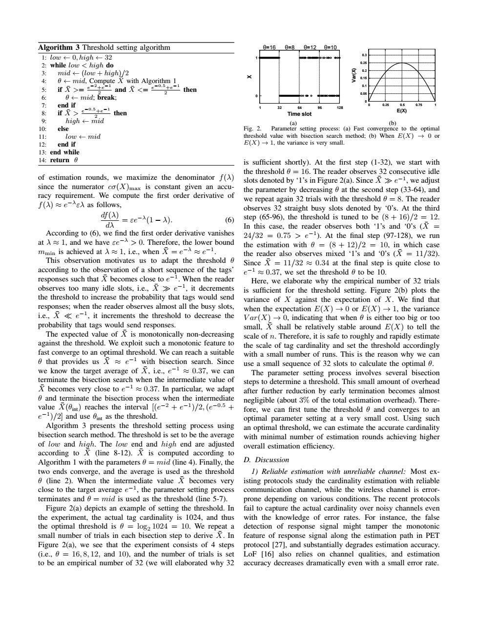When the reader observes too many idle slots, i.e., X¯  e −1 , it decrements the threshold to increase the probability that tags would send responses; when the reader observes almost all the busy slots, i.e., X¯  e −1 , it increments the threshold to decrease the probability that tags would send responses. The expected value of X¯ is monotonically non-decreasing against the threshold. We exploit such a monotonic feature to fast converge to an optimal threshold. We can reach a suitable θ that provides us X¯ ≈ e −1 with bisection search. Since we know the target average of X¯, i.e., e −1 ≈ 0.37, we can terminate the bisection search when the intermediate value of X¯ becomes very close to e −1 ≈ 0.37. In particular, we adapt θ and terminate the bisection process when the intermediate value X¯(θint) reaches the interval [(e −2 + e −1 )/2,(e −0.5 + e −1 )/2] and use θint as the threshold. Algorithm 3 presents the threshold setting process using bisection search method. The threshold is set to be the average of low and high. The low end and high end are adjusted according to X¯ (line 8-12). X¯ is computed according to Algorithm 1 with the parameters θ = mid (line 4). Finally, the two ends converge, and the average is used as the threshold θ (line 2). When the intermediate value X¯ becomes very close to the target average e −1 , the parameter setting process terminates and θ = mid is used as the threshold (line 5-7). Figure 2(a) depicts an example of setting the threshold. In the experiment, the actual tag cardinality is 1024, and thus the optimal threshold is θ = log2 1024 = 10. We repeat a small number of trials in each bisection step to derive X¯. In Figure 2(a), we see that the experiment consists of 4 steps (i.e., θ = 16, 8, 12, and 10), and the number of trials is set to be an empirical number of 32 (we will elaborated why 32 0 1 1 32 64 96 128 X Time slot θ=16 θ=8 θ=12 θ=10 (a) 0 0.05 0.1 0.15 0.2 0.25 0.3 0 0.25 0.5 0.75 1 Var(X) E(X) (b) Fig. 2. Parameter setting process: (a) Fast convergence to the optimal threshold value with bisection search method; (b) When E(X) → 0 or E(X) → 1, the variance is very small. is sufficient shortly). At the first step (1-32), we start with the threshold θ = 16. The reader observes 32 consecutive idle slots denoted by ‘1’s in Figure 2(a). Since X¯  e −1 , we adjust the parameter by decreasing θ at the second step (33-64), and we repeat again 32 trials with the threshold θ = 8. The reader observes 32 straight busy slots denoted by ‘0’s. At the third step (65-96), the threshold is tuned to be (8 + 16)/2 = 12. In this case, the reader observes both ‘1’s and ‘0’s (X¯ = 24/32 = 0.75 > e−1 ). At the final step (97-128), we run the estimation with θ = (8 + 12)/2 = 10, in which case the reader also observes mixed ‘1’s and ‘0’s (X¯ = 11/32). Since X¯ = 11/32 ≈ 0.34 at the final step is quite close to e −1 ≈ 0.37, we set the threshold θ to be 10. Here, we elaborate why the empirical number of 32 trials is sufficient for the threshold setting. Figure 2(b) plots the variance of X against the expectation of X. We find that when the expectation E(X) → 0 or E(X) → 1, the variance V ar(X) → 0, indicating that when θ is either too big or too small, X¯ shall be relatively stable around E(X) to tell the scale of n. Therefore, it is safe to roughly and rapidly estimate the scale of tag cardinality and set the threshold accordingly with a small number of runs. This is the reason why we can use a small sequence of 32 slots to calculate the optimal θ. The parameter setting process involves several bisection steps to determine a threshold. This small amount of overhead after further reduction by early termination becomes almost negligible (about 3% of the total estimation overhead). There￾fore, we can first tune the threshold θ and converges to an optimal parameter setting at a very small cost. Using such an optimal threshold, we can estimate the accurate cardinality with minimal number of estimation rounds achieving higher overall estimation efficiency. D. Discussion 1) Reliable estimation with unreliable channel: Most ex￾isting protocols study the cardinality estimation with reliable communication channel, while the wireless channel is error￾prone depending on various conditions. The recent protocols fail to capture the actual cardinality over noisy channels even with the knowledge of error rates. For instance, the false detection of response signal might tamper the monotonic feature of response signal along the estimation path in PET protocol [27], and substantially degrades estimation accuracy. LoF [16] also relies on channel qualities, and estimation accuracy decreases dramatically even with a small error rate