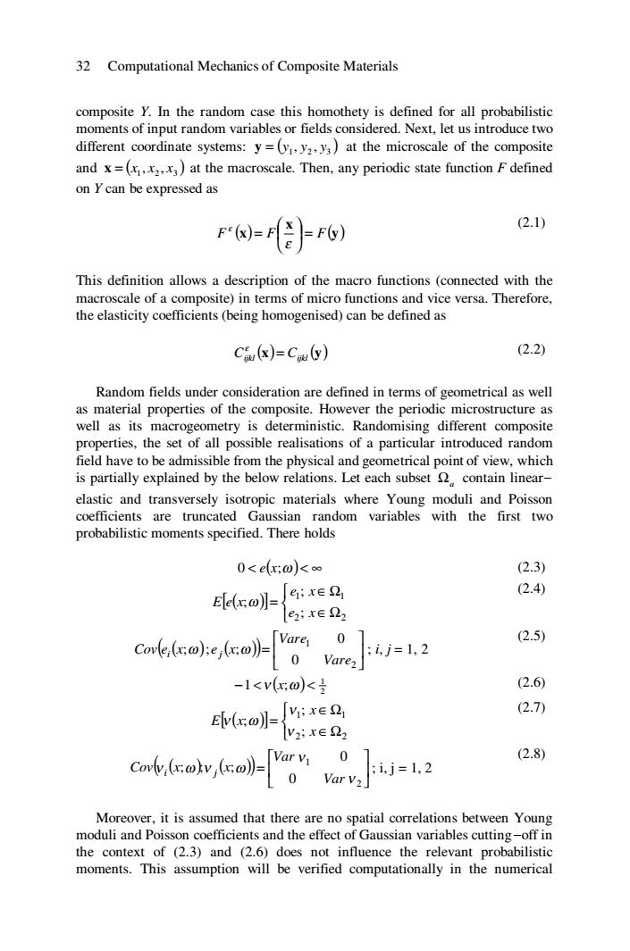
32 Computational Mechanics of Composite Materials composite Y.In the random case this homothety is defined for all probabilistic moments of input random variables or fields considered.Next,let us introduce two different coordinate systems:y=(yy2,y3)at the microscale of the composite and x=()at the macroscale.Then,any periodic state function F defined on Ycan be expressed as F(x)=F (2.1) This definition allows a description of the macro functions (connected with the macroscale of a composite)in terms of micro functions and vice versa.Therefore, the elasticity coefficients(being homogenised)can be defined as Ciu(x)=Cu(y) (2.2) Random fields under consideration are defined in terms of geometrical as well as material properties of the composite.However the periodic microstructure as well as its macrogeometry is deterministic.Randomising different composite properties,the set of all possible realisations of a particular introduced random field have to be admissible from the physical and geometrical point of view,which is partially explained by the below relations.Let each subset contain linear- elastic and transversely isotropic materials where Young moduli and Poisson coefficients are truncated Gaussian random variables with the first two probabilistic moments specified.There holds 0<e(ro)k∞ (2.3) Ele(co)= e1;x∈2 (2.4) e;xED2 cm(ak( 2.5) -1<v(co)< (2.6 E(co明=：xe (2.7) V2;x∈22 c(c(c (2.8) Moreover,it is assumed that there are no spatial correlations between Young moduli and Poisson coefficients and the effect of Gaussian variables cutting-off in the context of (2.3)and (2.6)does not influence the relevant probabilistic moments.This assumption will be verified computationally in the numerical32 Computational Mechanics of Composite Materials composite Y. In the random case this homothety is defined for all probabilistic moments of input random variables or fields considered. Next, let us introduce two different coordinate systems: ( ) 1 2 3 y = y , y , y at the microscale of the composite and ( ) 1 2 3 x = x , x , x at the macroscale. Then, any periodic state function F defined on Y can be expressed as ( ) ( ) y x F x F ⎟ = F ⎠ ⎞ ⎜ ⎝ ⎛ = ε ε (2.1) This definition allows a description of the macro functions (connected with the macroscale of a composite) in terms of micro functions and vice versa. Therefore, the elasticity coefficients (being homogenised) can be defined as () () x y Cijkl = Cijkl ε (2.2) Random fields under consideration are defined in terms of geometrical as well as material properties of the composite. However the periodic microstructure as well as its macrogeometry is deterministic. Randomising different composite properties, the set of all possible realisations of a particular introduced random field have to be admissible from the physical and geometrical point of view, which is partially explained by the below relations. Let each subset Ωa contain linear￾elastic and transversely isotropic materials where Young moduli and Poisson coefficients are truncated Gaussian random variables with the first two probabilistic moments specified. There holds 0 < e( ) x;ω < ∞ (2.3) [ ] ( ) ⎩ ⎨ ⎧ ∈Ω ∈Ω = 2 2 1 1 ; ; ; e x e x E e x ω (2.4) ( ) ( )( ) ⎥ ⎦ ⎤ ⎢ ⎣ ⎡ = 2 1 0 0 ; ; ; Vare Vare Cov e x e x i ω j ω ; i, j = 1, 2 (2.5) ( ) 2 1 −1 <ν x;ω < (2.6) [ ] ( ) ⎩ ⎨ ⎧ ∈Ω ∈Ω = 2 2 1 1 ; ; ; x x E x ν ν ν ω (2.7) ( ) ( )( ) ⎥ ⎦ ⎤ ⎢ ⎣ ⎡ = 2 1 0 0 ; ; ; ν ν ν ω ν ω Var Var Cov x x i j ; i, j = 1, 2 (2.8) Moreover, it is assumed that there are no spatial correlations between Young moduli and Poisson coefficients and the effect of Gaussian variables cutting-off in the context of (2.3) and (2.6) does not influence the relevant probabilistic moments. This assumption will be verified computationally in the numerical