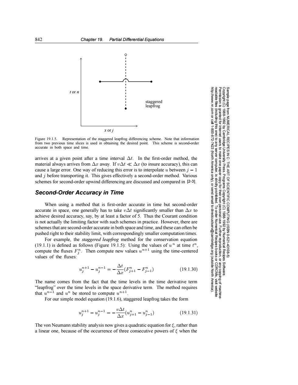
842 Chapter 19.Partial Differential Equations 0 staggered leapfrog 83 granted for x or j 1100 Figure 19.1.5.Representation of the staggered leapfrog differencing scheme.Note that information from two previous time slices is used in obtaining the desired point.This scheme is second-order NUMERICAL RECIPES I accurate in both space and time. arrives at a given point after a time interval At.In the first-order method,the material always arrives from Ax away.If vAtAx (to insure accuracy),this can cause a large error.One way of reducing this error is to interpolate u between i-1 2 and j before transporting it.This gives effectively a second-order method.Various schemes for second-order upwind differencing are discussed and compared in [2-3]. 9」 Second-Order Accuracy in Time IENTIFIC When using a method that is first-order accurate in time but second-order accurate in space,one generally has to take vAt significantly smaller than Ax to achieve desired accuracy,say,by at least a factor of 5.Thus the Courant condition is not actually the limiting factor with such schemes in practice.However,there are schemes that are second-order accurate in both space and time,and these can often be pushed right to their stability limit,with correspondingly smaller computation times. For example,the staggered leapfrog method for the conservation equation 10.621 (19.1.1)is defined as follows(Figure 19.1.5):Using the values of u at time t", Recipes Numerica compute the fluxesF".Then compute new values u+using the time-centered 431 values of the fluxes: Recipes 1-g写1=-g1-厚） (19.1.30 North The name comes from the fact that the time levels in the time derivative term "leapfrog"over the time levels in the space derivative term.The method requires that u"-1 and u"be stored to compute un+1. For our simple model equation(19.1.6),staggered leapfrog takes the form v△t +1-u-1=- (19.1.31) △x u+1-u巧-1) The von Neumann stability analysis now gives a quadratic equation for rather than a linear one,because of the occurrence of three consecutive powers ofg when the842 Chapter 19. Partial Differential Equations Permission is granted for internet users to make one paper copy for their own personal use. Further reproduction, or any copyin Copyright (C) 1988-1992 by Cambridge University Press. Programs Copyright (C) 1988-1992 by Numerical Recipes Software. Sample page from NUMERICAL RECIPES IN C: THE ART OF SCIENTIFIC COMPUTING (ISBN 0-521-43108-5) g of machine￾readable files (including this one) to any server computer, is strictly prohibited. To order Numerical Recipes books or CDROMs, visit website http://www.nr.com or call 1-800-872-7423 (North America only), or send email to directcustserv@cambridge.org (outside North America). staggered leapfrog t or n x or j Figure 19.1.5. Representation of the staggered leapfrog differencing scheme. Note that information from two previous time slices is used in obtaining the desired point. This scheme is second-order accurate in both space and time. arrives at a given point after a time interval ∆t. In the first-order method, the material always arrives from ∆x away. If v∆t ∆x (to insure accuracy), this can cause a large error. One way of reducing this error is to interpolate u between j − 1 and j before transporting it. This gives effectively a second-order method. Various schemes for second-order upwind differencing are discussed and compared in [2-3]. Second-Order Accuracy in Time When using a method that is first-order accurate in time but second-order accurate in space, one generally has to take v∆t significantly smaller than ∆x to achieve desired accuracy, say, by at least a factor of 5. Thus the Courant condition is not actually the limiting factor with such schemes in practice. However, there are schemes that are second-order accurate in both space and time, and these can often be pushed right to their stability limit, with correspondingly smaller computation times. For example, the staggered leapfrog method for the conservation equation (19.1.1) is defined as follows (Figure 19.1.5): Using the values of u n at time tn, compute the fluxes F n j . Then compute new values un+1 using the time-centered values of the fluxes: un+1 j − un−1 j = − ∆t ∆x(F n j+1 − F n j−1) (19.1.30) The name comes from the fact that the time levels in the time derivative term “leapfrog” over the time levels in the space derivative term. The method requires that un−1 and un be stored to compute un+1. For our simple model equation (19.1.6), staggered leapfrog takes the form un+1 j − un−1 j = −v∆t ∆x (un j+1 − un j−1) (19.1.31) The von Neumann stability analysis now gives a quadratic equation for ξ, rather than a linear one, because of the occurrence of three consecutive powers of ξ when the