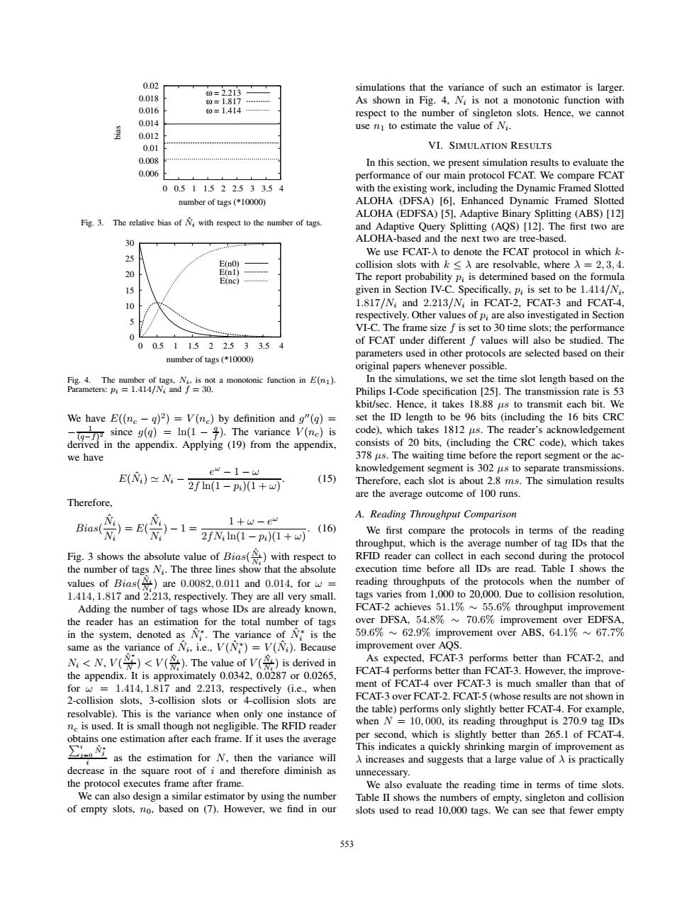
0.02 0=2.213 simulations that the variance of such an estimator is larger 0.018 0=1.817… As shown in Fig.4,Ni is not a monotonic function with 0.016 0=1.414… respect to the number of singleton slots.Hence,we cannot 0.014 use n to estimate the value of Ni. 0.012 0.01 VI.SIMULATION RESULTS 0.008 In this section,we present simulation results to evaluate the 0.006 performance of our main protocol FCAT.We compare FCAT 00.511.522.533.54 with the existing work,including the Dynamic Framed Slotted number of tags (*10000) ALOHA (DFSA)[6].Enhanced Dynamic Framed Slotted ALOHA (EDFSA)[5],Adaptive Binary Splitting (ABS)[12] Fig.3. The relative bias of with respect to the number of tags. and Adaptive Query Splitting (AQS)[12].The first two are 30 ALOHA-based and the next two are tree-based. We use FCAT-A to denote the FCAT protocol in which k- 25 E(n0) collision slots withk≤入are resolvable,where入=2,3,4. 20 E(n1) E(nC）a The report probability p;is determined based on the formula 15 given in Section IV-C.Specifically,p;is set to be 1.414/Ni. 1.817/N;and 2.213/N;in FCAT-2.FCAT-3 and FCAT-4. respectively.Other values of p;are also investigated in Section VI-C.The frame size f is set to 30 time slots;the performance 0￥ of FCAT under different f values will also be studied.The 00.511.522.533.54 number of tags (*10000) parameters used in other protocols are selected based on their original papers whenever possible. Fig.4.The number of tags.N.is not a monotonic function in E(n). In the simulations,we set the time slot length based on the Parameters:pi 1.414/Ni and f=30. Philips I-Code specification [25].The transmission rate is 53 kbit/sec.Hence,it takes 18.88 us to transmit each bit.We We have E((ne-q)2)=V(ne)by definition and g"(q)= set the ID length to be 96 bits (including the 16 bits CRC i高(m te sp code),which takes 1812 us.The reader's acknowledgement consists of 20 bits,(including the CRC code),which takes we have 378 us.The waiting time before the report segment or the ac- e“-1-d knowledgement segment is 302 us to separate transmissions. E()≈N:- 2fm(1-p)(1+w) (15) Therefore,each slot is about 2.8 ms.The simulation results are the average outcome of 100 runs. Therefore. A.Reading Throughput Comparison Bias( 1+w-e“ (16) 2fNn(1-p)(1+w) We first compare the protocols in terms of the reading throughput,which is the average number of tag IDs that the Fig.3 shows the absolute value of Bias()with respect to RFID reader can collect in each second during the protocol the number of tags N:.The three lines show that the absolute execution time before all IDs are read.Table I shows the values of Bias()are 0.0082,0.011 and 0.014,for w= reading throughputs of the protocols when the number of 1.414,1.817 and 2.213,respectively.They are all very small. tags varies from 1,000 to 20,000.Due to collision resolution, Adding the number of tags whose IDs are already known, FCAT-2 achieves 51.1%~55.6%throughput improvement the reader has an estimation for the total number of tags over DFSA,54.8%~70.6%improvement over EDFSA, in the system,denoted as N.The variance of N*is the 59.6%62.9%improvement over ABS,64.1%~67.7% same as the variance of Ni.i.e.,V(N)=V(Ni).Because improvement over AQS. N:<N.V()<V().The value of V()is derived in As expected,FCAT-3 performs better than FCAT-2,and the appendix.It is approximately 0.0342,0.0287 or 0.0265, FCAT-4 performs better than FCAT-3.However,the improve- for w 1.414,1.817 and 2.213,respectively (i.e.,when ment of FCAT-4 over FCAT-3 is much smaller than that of 2-collision slots,3-collision slots or 4-collision slots are FCAT-3 over FCAT-2.FCAT-5(whose results are not shown in resolvable).This is the variance when only one instance of the table)performs only slightly better FCAT-4.For example, ne is used.It is small though not negligible.The RFID reader when N 10,000,its reading throughput is 270.9 tag IDs obtains one estimation after each frame.If it uses the average per second,which is slightly better than 265.1 of FCAT-4. as the estimation for N.then the variancewill This indicates a quickly shrinking margin of improvement as A increases and suggests that a large value of A is practically decrease in the square root of i and therefore diminish as unnecessary. the protocol executes frame after frame We also evaluate the reading time in terms of time slots. We can also design a similar estimator by using the number Table II shows the numbers of empty,singleton and collision of empty slots,no,based on (7).However,we find in our slots used to read 10,000 tags.We can see that fewer empty 5530.006 0.008 0.01 0.012 0.014 0.016 0.018 0.02 0 0.5 1 1.5 2 2.5 3 3.5 4 bias number of tags (*10000) ω = 2.213 ω = 1.817 ω = 1.414 Fig. 3. The relative bias of Nˆi with respect to the number of tags. 0 5 10 15 20 25 30 0 0.5 1 1.5 2 2.5 3 3.5 4 number of tags (*10000) E(n0) E(n1) E(nc) Fig. 4. The number of tags, Ni, is not a monotonic function in E(n1). Parameters: pi = 1.414/Ni and f = 30. We have E((nc − q)2) = V (nc) by definition and g(q) = − 1 (q−f)2 since g(q) = ln(1 − q f ). The variance V (nc) is derived in the appendix. Applying (19) from the appendix, we have E(Nˆi) Ni − eω − 1 − ω 2f ln(1 − pi)(1 + ω) . (15) Therefore, Bias( Nˆi Ni ) = E( Nˆi Ni ) − 1 = 1 + ω − eω 2fNi ln(1 − pi)(1 + ω) . (16) Fig. 3 shows the absolute value of Bias( Nˆi Ni ) with respect to the number of tags Ni. The three lines show that the absolute values of Bias( Nˆi Ni ) are 0.0082, 0.011 and 0.014, for ω = 1.414, 1.817 and 2.213, respectively. They are all very small. Adding the number of tags whose IDs are already known, the reader has an estimation for the total number of tags in the system, denoted as Nˆ ∗ i . The variance of Nˆ ∗ i is the same as the variance of Nˆi, i.e., V (Nˆ ∗ i ) = V (Nˆi). Because Ni < N, V ( Nˆ ∗ i N ) < V ( Nˆi Ni ). The value of V ( Nˆi Ni ) is derived in the appendix. It is approximately 0.0342, 0.0287 or 0.0265, for ω = 1.414, 1.817 and 2.213, respectively (i.e., when 2-collision slots, 3-collision slots or 4-collision slots are resolvable). This is the variance when only one instance of nc is used. It is small though not negligible. The RFID reader obtains one estimation after each frame. If it uses the average i j=0 Nˆ ∗ j i as the estimation for N, then the variance will decrease in the square root of i and therefore diminish as the protocol executes frame after frame. We can also design a similar estimator by using the number of empty slots, n0, based on (7). However, we find in our simulations that the variance of such an estimator is larger. As shown in Fig. 4, Ni is not a monotonic function with respect to the number of singleton slots. Hence, we cannot use n1 to estimate the value of Ni. VI. SIMULATION RESULTS In this section, we present simulation results to evaluate the performance of our main protocol FCAT. We compare FCAT with the existing work, including the Dynamic Framed Slotted ALOHA (DFSA) [6], Enhanced Dynamic Framed Slotted ALOHA (EDFSA) [5], Adaptive Binary Splitting (ABS) [12] and Adaptive Query Splitting (AQS) [12]. The first two are ALOHA-based and the next two are tree-based. We use FCAT-λ to denote the FCAT protocol in which k￾collision slots with k ≤ λ are resolvable, where λ = 2, 3, 4. The report probability pi is determined based on the formula given in Section IV-C. Specifically, pi is set to be 1.414/Ni, 1.817/Ni and 2.213/Ni in FCAT-2, FCAT-3 and FCAT-4, respectively. Other values of pi are also investigated in Section VI-C. The frame size f is set to 30 time slots; the performance of FCAT under different f values will also be studied. The parameters used in other protocols are selected based on their original papers whenever possible. In the simulations, we set the time slot length based on the Philips I-Code specification [25]. The transmission rate is 53 kbit/sec. Hence, it takes 18.88 μs to transmit each bit. We set the ID length to be 96 bits (including the 16 bits CRC code), which takes 1812 μs. The reader’s acknowledgement consists of 20 bits, (including the CRC code), which takes 378 μs. The waiting time before the report segment or the ac￾knowledgement segment is 302 μs to separate transmissions. Therefore, each slot is about 2.8 ms. The simulation results are the average outcome of 100 runs. A. Reading Throughput Comparison We first compare the protocols in terms of the reading throughput, which is the average number of tag IDs that the RFID reader can collect in each second during the protocol execution time before all IDs are read. Table I shows the reading throughputs of the protocols when the number of tags varies from 1,000 to 20,000. Due to collision resolution, FCAT-2 achieves 51.1% ∼ 55.6% throughput improvement over DFSA, 54.8% ∼ 70.6% improvement over EDFSA, 59.6% ∼ 62.9% improvement over ABS, 64.1% ∼ 67.7% improvement over AQS. As expected, FCAT-3 performs better than FCAT-2, and FCAT-4 performs better than FCAT-3. However, the improve￾ment of FCAT-4 over FCAT-3 is much smaller than that of FCAT-3 over FCAT-2. FCAT-5 (whose results are not shown in the table) performs only slightly better FCAT-4. For example, when N = 10, 000, its reading throughput is 270.9 tag IDs per second, which is slightly better than 265.1 of FCAT-4. This indicates a quickly shrinking margin of improvement as λ increases and suggests that a large value of λ is practically unnecessary. We also evaluate the reading time in terms of time slots. Table II shows the numbers of empty, singleton and collision slots used to read 10,000 tags. We can see that fewer empty 553