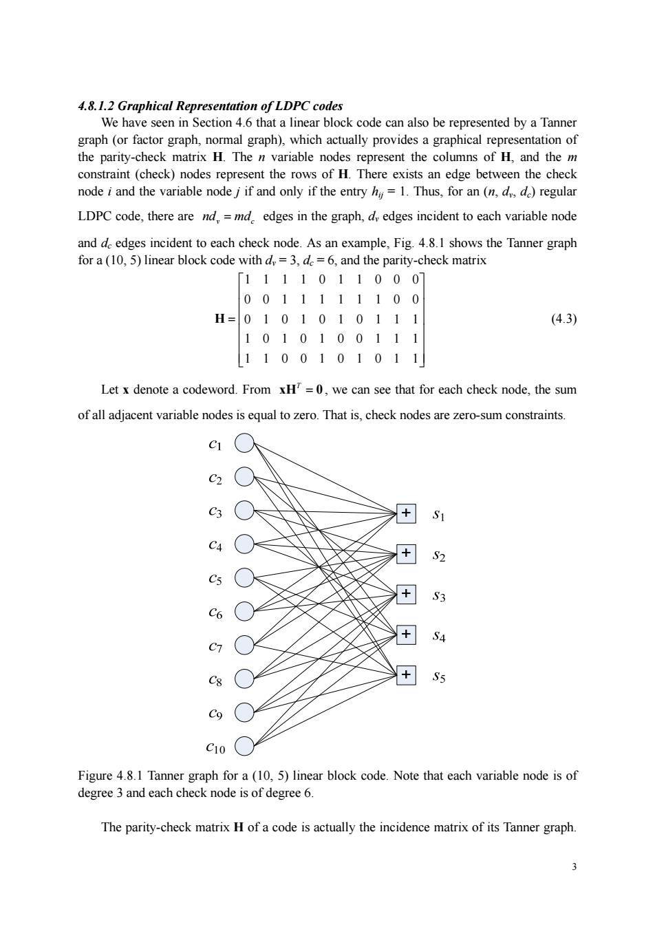
have seen in ection 4.6 that a linear block code can also be represented by aTanne graph (or factor graph,normal graph),which actually provides a graphical representation of the parity-check matrix H.The n variable nodes represent the columns of H,and the m constraint(check)nodes represent the rows of H.There exists an edge between the check node i and the variable node j if and only if the entryh=1.Thus,for an (n,dd)regular LDPC code,there are nd,=md edges in the graph,d,edges incident to each variable node and d edges incident to each check node.As an example,Fig.4.8.1 shows the Tanner graph for a (10,5)linear block code withd=3,de=6,and the parity-check matrix [11110110 00] 0011111100 H=0101010111 (4.3) 1010100111 1100101011 Let x denote a codeword.From xH=0,we can see that for each check node,the sum of all adjacent variable nodes is equal to zero.That is,check nodes are zero-sum constraints. C3 + S1 C4 S2 + S3 + S4 S5 cg○ Figure 4.8.1 Tanner graph for a(10,5)linear block code.Note that each variable node is of degree 3 and each check node is of degree 6. The parity-check matrix H of a code is actually the incidence matrix of its Tanner graph 33 4.8.1.2 Graphical Representation of LDPC codes We have seen in Section 4.6 that a linear block code can also be represented by a Tanner graph (or factor graph, normal graph), which actually provides a graphical representation of the parity-check matrix H. The n variable nodes represent the columns of H, and the m constraint (check) nodes represent the rows of H. There exists an edge between the check node i and the variable node j if and only if the entry hij = 1. Thus, for an (n, dv, dc) regular LDPC code, there are v c nd md = edges in the graph, dv edges incident to each variable node and dc edges incident to each check node. As an example, Fig. 4.8.1 shows the Tanner graph for a (10, 5) linear block code with dv = 3, dc = 6, and the parity-check matrix 1111011000 0011111100 0101010111 1010100111 1100101011 ⎡ ⎤ ⎢ ⎥ = ⎣ ⎦ H (4.3) Let x denote a codeword. From T xH 0 = , we can see that for each check node, the sum of all adjacent variable nodes is equal to zero. That is, check nodes are zero-sum constraints. Figure 4.8.1 Tanner graph for a (10, 5) linear block code. Note that each variable node is of degree 3 and each check node is of degree 6. The parity-check matrix H of a code is actually the incidence matrix of its Tanner graph