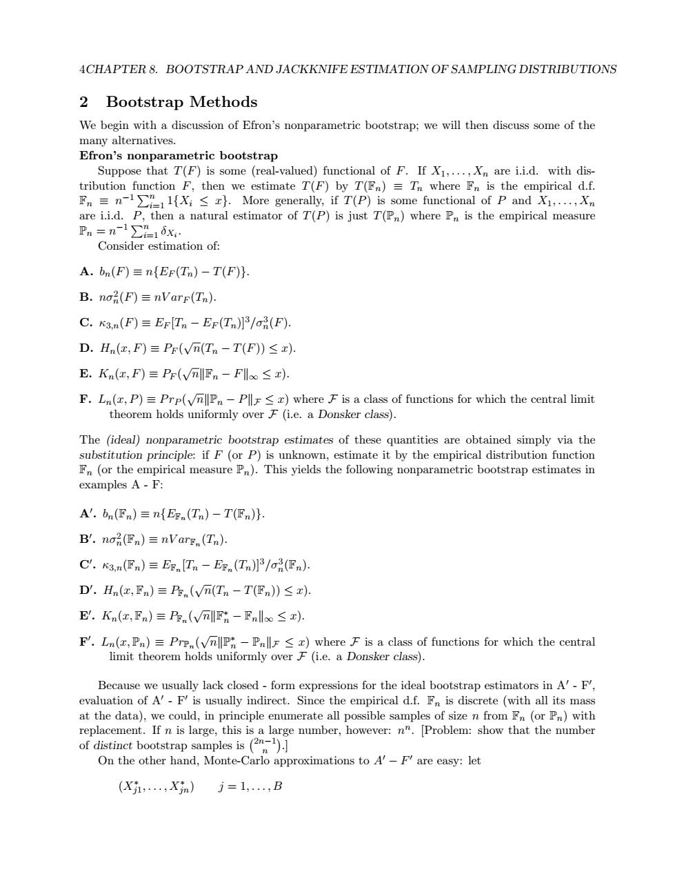
4CHAPTER 8.BOOTSTRAP AND JACKKNIFE ESTIMATION OF SAMPLING DISTRIBUTIONS 2 Bootstrap Methods We begin with a discussion of Efron's nonparametric bootstrap;we will then discuss some of the many alternatives. Efron's nonparametric bootstrap Suppose that T(F)is some (real-valued)functional of F.If X1,...,Xn are i.i.d.with dis- tribution function F,then we estimate T(F)by T(Fn)=Tn where Fn is the empirical d.f. Fn=n-1 )More generally,if T(P)is some functional of P and X1,...,Xn are i.i.d.P,then a natural estimator of T(P)is just T(Pn)where Pn is the empirical measure Pn=n-1∑g1dx: Consider estimation of: A.bn(F)=nEF(Tn)-T(F). B.no2(F)≡nVarF(Tn). C.K3.n(F)=EF[Tn-EF(Tn)]3/n(F). D.Hn(x,F)=Pr(Vn(Tn-T(F))<). E.Kn(c,F)≡Pr(√nFn-Flo≤x) F.Ln(,P)=Prp(vnPn-Px)where F is a class of functions for which the central limit theorem holds uniformly over F(i.e.a Donsker class). The (ideal)nonparametric bootstrap estimates of these quantities are obtained simply via the substitution principle:if F(or P)is unknown,estimate it by the empirical distribution function Fn(or the empirical measure Pn).This yields the following nonparametric bootstrap estimates in examples A-F: A'.bn(Fn)=nfEEn (Tn)-T(Fn)} B'.noi(Fn)=nVarg,(Tn). C/.K3.n(Fn)=Eg [Tn-EF (Tn)]3/on(Fn). D'.Hn(a,Fn)≡Pgn(m(Tn-T(fn)≤x): E'.Kn(x,Fn)≡Pgn(VFt-Fnlo≤x) F'.Ln(,Pn)=Prp (vnlPh -PnllF x)where F is a class of functions for which the central limit theorem holds uniformly over F(i.e.a Donsker class). Because we usually lack closed-form expressions for the ideal bootstrap estimators in A'-F, evaluation of A'-F is usually indirect.Since the empirical d.f.Fn is discrete (with all its mass at the data),we could,in principle enumerate all possible samples of size n from Fn(or Pn)with replacement.If n is large,this is a large number,however:n".Problem:show that the number of distinct bootstrap samples is(] On the other hand,Monte-Carlo approximations to A'-F are easy:let (X1,,Xjm)j=1,,B4CHAPTER 8. BOOTSTRAP AND JACKKNIFE ESTIMATION OF SAMPLING DISTRIBUTIONS 2 Bootstrap Methods We begin with a discussion of Efron’s nonparametric bootstrap; we will then discuss some of the many alternatives. Efron’s nonparametric bootstrap Suppose that T(F) is some (real-valued) functional of F. If X1, . . . , Xn are i.i.d. with dis￾tribution function F, then we estimate T(F) by T(Fn) ≡ Tn where Fn is the empirical d.f. Fn ≡ n −1 Pn i=1 1{Xi ≤ x}. More generally, if T(P) is some functional of P and X1, . . . , Xn are i.i.d. P, then a natural estimator of T(P) is just T(Pn) where Pn is the empirical measure Pn = n −1 Pn i=1 δXi . Consider estimation of: A. bn(F) ≡ n{EF (Tn) − T(F)}. B. nσ2 n (F) ≡ nV arF (Tn). C. κ3,n(F) ≡ EF [Tn − EF (Tn)]3/σ3 n (F). D. Hn(x, F) ≡ PF ( √ n(Tn − T(F)) ≤ x). E. Kn(x, F) ≡ PF ( √ nkFn − Fk∞ ≤ x). F. Ln(x, P) ≡ P rP ( √ nkPn − PkF ≤ x) where F is a class of functions for which the central limit theorem holds uniformly over F (i.e. a Donsker class). The (ideal) nonparametric bootstrap estimates of these quantities are obtained simply via the substitution principle: if F (or P) is unknown, estimate it by the empirical distribution function Fn (or the empirical measure Pn). This yields the following nonparametric bootstrap estimates in examples A - F: A0 . bn(Fn) ≡ n{EFn (Tn) − T(Fn)}. B0 . nσ2 n (Fn) ≡ nV arFn (Tn). C0 . κ3,n(Fn) ≡ EFn [Tn − EFn (Tn)]3/σ3 n (Fn). D0 . Hn(x, Fn) ≡ PFn ( √ n(Tn − T(Fn)) ≤ x). E0 . Kn(x, Fn) ≡ PFn ( √ nkF ∗ n − Fnk∞ ≤ x). F 0 . Ln(x, Pn) ≡ P rPn ( √ nkP ∗ n − PnkF ≤ x) where F is a class of functions for which the central limit theorem holds uniformly over F (i.e. a Donsker class). Because we usually lack closed - form expressions for the ideal bootstrap estimators in A0 - F0 , evaluation of A0 - F0 is usually indirect. Since the empirical d.f. Fn is discrete (with all its mass at the data), we could, in principle enumerate all possible samples of size n from Fn (or Pn) with replacement. If n is large, this is a large number, however: n n . [Problem: show that the number of distinct bootstrap samples is ￾ 2n−1 n
.] On the other hand, Monte-Carlo approximations to A0 − F 0 are easy: let (X∗ j1 , . . . , X∗ jn) j = 1, . . . , B