正在加载图片...

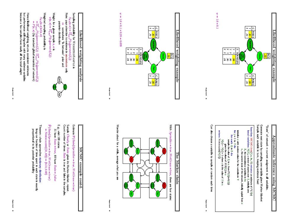
ea few samples have nearly all the total weight "prior and Likelihood weighting analysis Likelihood weighting example 色88 Likelihood weighting example ! Wander about MCMC example contd. fre,there are four state The Markov chain Can aso choose a variable to sample at random each time Approximate inference using MCMCLikelihood weighting example Cloudy Rain Sprinkler Grass Wet F T C .20 .80 P(R|C) F T C .50 .10 P(S|C) S R T T T F F T F F .90 .90 .99 P(W|S,R) P(C) .50 .01 w = 1.0 × 0.1 Chapter 14.4–5 31 Likelihood weighting example Cloudy Rain Sprinkler Grass Wet F T C .20 .80 P(R|C) F T C .50 .10 P(S|C) S R T T T F F T F F .90 .90 .99 P(W|S,R) P(C) .50 .01 w = 1.0 × 0.1 × 0.99 = 0.099 Chapter 14.4–5 32 Likelihood weighting analysis Sampling probability for WeightedSample is SWS(z, e) = Πi l = 1P(zi |parents(Zi)) Note: pays attention to evidence in ancestors only Cloudy Rain Sprinkler Grass Wet ⇒ somewhere “in between” prior and posterior distribution Weight for a given sample z, e is w(z, e) = Πi m = 1P(ei |parents(Ei)) Weighted sampling probability is SWS(z, e)w(z, e) = Πi l = 1P(zi |parents(Zi)) Πi m = 1P(ei |parents(Ei)) = P(z, e) (by standard global semantics of network) Hence likelihood weighting returns consistent estimates but performance still degrades with many evidence variables because a few samples have nearly all the total weight Chapter 14.4–5 33 Approximate inference using MCMC “State” of network = current assignment to all variables. Generate next state by sampling one variable given Markov blanket Sample each variable in turn, keeping evidence fixed function MCMC-Ask(X, e, bn,N) returns an estimate of P(X |e) local variables: N[X ], a vector of counts over X, initially zero Z, the nonevidence variables in bn x, the current state of the network, initially copied from e initialize x with random values for the variables in Y for j = 1 to N do for each Zi in Z do sample the value of Zi in x from P(Zi|mb(Zi)) given the values of MB(Zi) in x N[x ] ← N[x ] + 1 where x is the value of X in x return Normalize(N[X ]) Can also choose a variable to sample at random each time Chapter 14.4–5 34 The Markov chain With Sprinkler = true, WetGrass = true, there are four states: Cloudy Rain Sprinkler Grass Wet Cloudy Rain Sprinkler Grass Wet Cloudy Rain Sprinkler Grass Wet Cloudy Rain Sprinkler Grass Wet Wander about for a while, average what you see Chapter 14.4–5 35 MCMC example contd. Estimate P(Rain|Sprinkler = true, WetGrass = true) Sample Cloudy or Rain given its Markov blanket, repeat. Count number of times Rain is true and false in the samples. E.g., visit 100 states 31 have Rain = true, 69 have Rain = false Pˆ (Rain|Sprinkler = true, WetGrass = true) = Normalize(h31, 69i) = h0.31, 0.69i Theorem: chain approaches stationary distribution: long-run fraction of time spent in each state is exactly proportional to its posterior probability Chapter 14.4–5 36