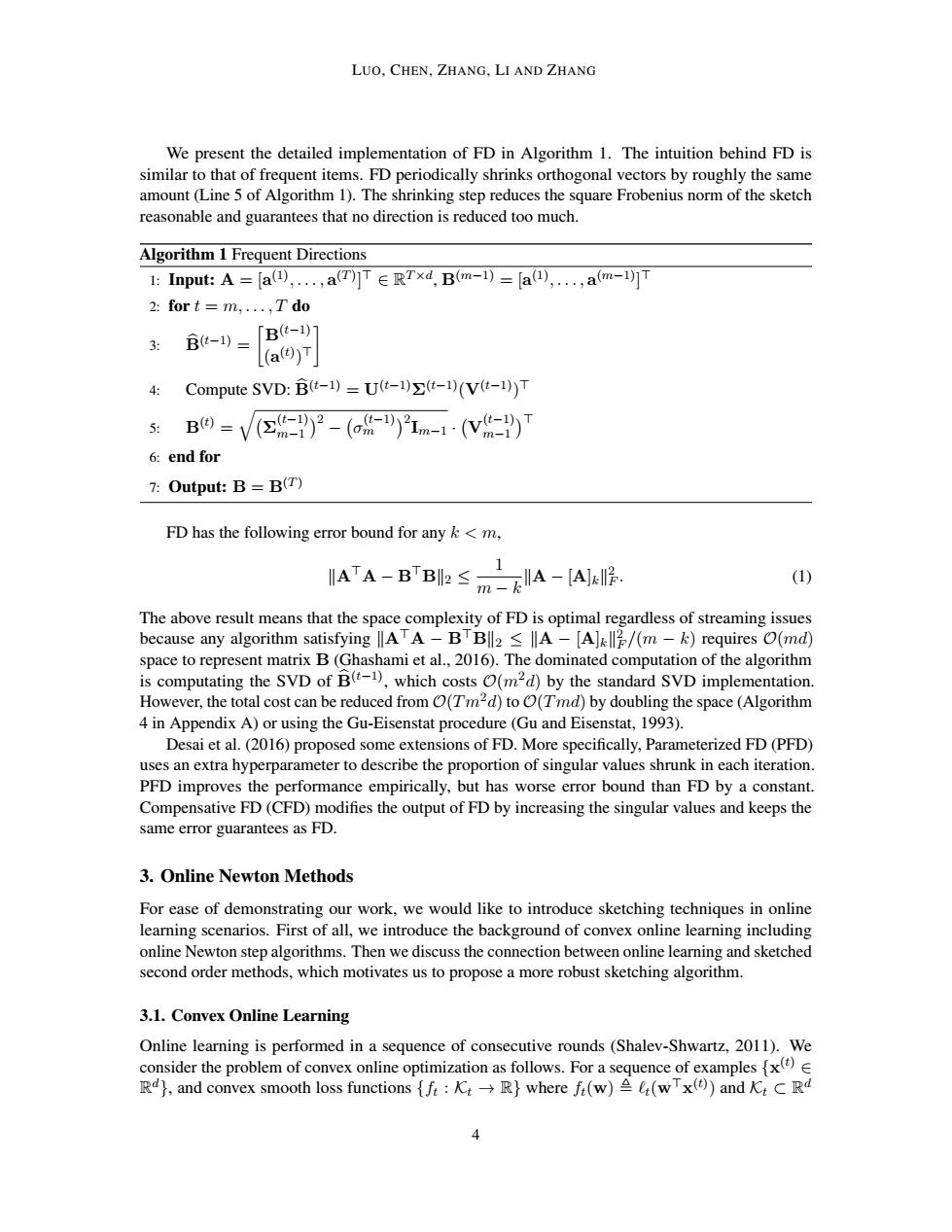
LUO.CHEN,ZHANG,LI AND ZHANG We present the detailed implementation of FD in Algorithm 1.The intuition behind FD is similar to that of frequent items.FD periodically shrinks orthogonal vectors by roughly the same amount(Line 5 of Algorithm 1).The shrinking step reduces the square Frobenius norm of the sketch reasonable and guarantees that no direction is reduced too much. Algorithm 1 Frequent Directions 1:Inputs:A=a四，.，aT)]TERTxd,Bm-)=a①..，am-]T 2:for t =m,...,T do 3: Bt-1)= 「B(t-1) (a())T Compute SVD:B(t-1)=U(t-1)>(t-1)(V(t-1))T B9=V(②-2-(og-)21m-·(v-)T 6:end for 7:Output:B=B(T) FD has the following error bound for any k<m, IATA-B'B≤m天A-Ae2 (1) The above result means that the space complexity of FD is optimal regardless of streaming issues because any algorithm satisfying ATA-BTBll2 A-[A](m-k)requires O(md) space to represent matrix B(Ghashami et al.,2016).The dominated computation of the algorithm is computating the SVD of B(-1),which costs (m2d)by the standard SVD implementation. However,the total cost can be reduced from (Tm2d)to (Tmd)by doubling the space (Algorithm 4 in Appendix A)or using the Gu-Eisenstat procedure(Gu and Eisenstat,1993). Desai et al.(2016)proposed some extensions of FD.More specifically,Parameterized FD(PFD) uses an extra hyperparameter to describe the proportion of singular values shrunk in each iteration. PFD improves the performance empirically,but has worse error bound than FD by a constant. Compensative FD(CFD)modifies the output of FD by increasing the singular values and keeps the same error guarantees as FD. 3.Online Newton Methods For ease of demonstrating our work,we would like to introduce sketching techniques in online learning scenarios.First of all,we introduce the background of convex online learning including online Newton step algorithms.Then we discuss the connection between online learning and sketched second order methods,which motivates us to propose a more robust sketching algorithm. 3.1.Convex Online Learning Online learning is performed in a sequence of consecutive rounds(Shalev-Shwartz,2011).We consider the problem of convex online optimization as follows.For a sequence of examples() Rd),and convex smooth loss functions {f:KR}where f(w)(wTx()and K:C Rd 4LUO, CHEN, ZHANG, LI AND ZHANG We present the detailed implementation of FD in Algorithm 1. The intuition behind FD is similar to that of frequent items. FD periodically shrinks orthogonal vectors by roughly the same amount (Line 5 of Algorithm 1). The shrinking step reduces the square Frobenius norm of the sketch reasonable and guarantees that no direction is reduced too much. Algorithm 1 Frequent Directions 1: Input: A = [a (1) , . . . , a (T) ] > ∈ R T ×d , B(m−1) = [a (1) , . . . , a (m−1)] > 2: for t = m, . . . , T do 3: Bb(t−1) =  B(t−1) (a (t) ) >  4: Compute SVD: Bb(t−1) = U(t−1)Σ(t−1)(V(t−1)) > 5: B(t) = q￾ Σ (t−1) m−1
2 − ￾ σ (t−1) m
2 Im−1 · ￾ V (t−1) m−1
> 6: end for 7: Output: B = B(T) FD has the following error bound for any k < m, kA>A − B >Bk2 ≤ 1 m − k kA − [A]kk 2 F . (1) The above result means that the space complexity of FD is optimal regardless of streaming issues because any algorithm satisfying kA>A − B>Bk2 ≤ kA − [A]kk 2 F /(m − k) requires O(md) space to represent matrix B (Ghashami et al., 2016). The dominated computation of the algorithm is computating the SVD of Bb(t−1), which costs O(m2d) by the standard SVD implementation. However, the total cost can be reduced from O(Tm2d) to O(Tmd) by doubling the space (Algorithm 4 in Appendix A) or using the Gu-Eisenstat procedure (Gu and Eisenstat, 1993). Desai et al. (2016) proposed some extensions of FD. More specifically, Parameterized FD (PFD) uses an extra hyperparameter to describe the proportion of singular values shrunk in each iteration. PFD improves the performance empirically, but has worse error bound than FD by a constant. Compensative FD (CFD) modifies the output of FD by increasing the singular values and keeps the same error guarantees as FD. 3. Online Newton Methods For ease of demonstrating our work, we would like to introduce sketching techniques in online learning scenarios. First of all, we introduce the background of convex online learning including online Newton step algorithms. Then we discuss the connection between online learning and sketched second order methods, which motivates us to propose a more robust sketching algorithm. 3.1. Convex Online Learning Online learning is performed in a sequence of consecutive rounds (Shalev-Shwartz, 2011). We consider the problem of convex online optimization as follows. For a sequence of examples {x (t) ∈ R d}, and convex smooth loss functions {ft : Kt → R} where ft(w) , `t(w>x (t) ) and Kt ⊂ R d 4