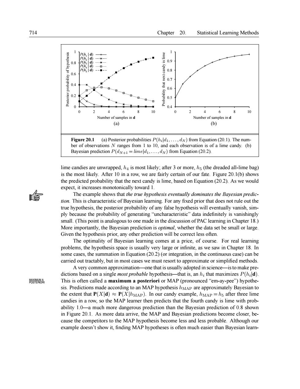
714 Chapter 20. Statistical Learning Methods 0.9 0 ◆ 0.8 。 0.6 0 8 0 10 les in les in d (a) Figure20.1 (a)Posterior probabilities P(hald1.. dy)from Equation(20.1).The num ber of observations N ranges from 1 to 10,and each observation is of a lime candy.(b) Bayesian prediction P(dN+=limeld....dN)from Equation(20.2). lime e candies ar unw apped,is most likely after 3 or more,(the dreaded all- ime bag is the most likely After In a row,we are fai 0.1(b)show the predi ted probability that the next candy is lime,based on Equation (20.2).As we would expec .it increas monotonically toward The example shows that the true hypothesis eventually dominates the Bayesian pred tion This is characteristic of Bayesian leaming.For any fixed prior that does not rule out the true hypothesis,the posterior probability ofany false hypothesis will eventually vanish,sim ply because the probability of generating "uncharacteristic"data indefinitely is vanishingl small.(This point is analogous to one made in the discussion of PAC learning in Chapter 18.) More importantly,the Bayesian prediction is oprimal,whether the data set be small or large. Given the hypothesis prior,any other prediction will be correct less often. The optimality of Bayesian learning comes at a price,of course.For real learning problems,the hypothesis space is usually very large or infinite,as we saw in Chapter 18.In some cases,the summation in Equation(20.2)(or integration,in the continuous case)can be carried out tractably,but in most cases we must resort to approximate or simplified methods. A very common approximation- -one that is usually adopted in science- -is to make pre dictions based on a single most probable hypothesis- that is,an h;that maximizes P(hd) A This is often called a maximum a posteriori or MAP (pronounced"em-ay-pee")hypothe- sis.Predictions made according to an MAP hypothesis hMAP are approximately Bayesian to the extent that P(XId)P(XMAP).In our candy example,hMAP=hs after three lime candies in a row.so the MAP learner then predicts that the fourth candy is lime with prob ability 1.0-a much more dangerous prediction than the Bayesian prediction of 0.8 shown in Figure 20.1.As more data arrive,the MAP and Bayesian predictions become closer,be- cause the competitors to the MAP hypothesis become less and less probable.Although our example doesn't show it,finding MAP hypotheses is often much easier than Bayesian learn- 714 Chapter 20. Statistical Learning Methods 0 0.2 0.4 0.6 0.8 1 0 2 4 6 8 10 Posterior probability of hypothesis Number of samples in d P(h1 | d) P(h2 | d) P(h3 | d) P(h4 | d) P(h5 | d) 0.4 0.5 0.6 0.7 0.8 0.9 1 0 2 4 6 8 10 Probability that next candy is lime Number of samples in d (a) (b) Figure 20.1 (a) Posterior probabilities P(hi |d1, . . . , dN ) from Equation (20.1). The num￾ber of observations N ranges from 1 to 10, and each observation is of a lime candy. (b) Bayesian prediction P(dN+1 = lime|d1, . . . , dN ) from Equation (20.2). lime candies are unwrapped, h4 is most likely; after 3 or more, h5 (the dreaded all-lime bag) is the most likely. After 10 in a row, we are fairly certain of our fate. Figure 20.1(b) shows the predicted probability that the next candy is lime, based on Equation (20.2). As we would expect, it increases monotonically toward 1. The example shows that the true hypothesis eventually dominates the Bayesian predic￾tion. This is characteristic of Bayesian learning. For any fixed prior that does not rule out the true hypothesis, the posterior probability of any false hypothesis will eventually vanish, sim￾ply because the probability of generating “uncharacteristic” data indefinitely is vanishingly small. (This point is analogous to one made in the discussion of PAC learning in Chapter 18.) More importantly, the Bayesian prediction is optimal, whether the data set be small or large. Given the hypothesis prior, any other prediction will be correct less often. The optimality of Bayesian learning comes at a price, of course. For real learning problems, the hypothesis space is usually very large or infinite, as we saw in Chapter 18. In some cases, the summation in Equation (20.2) (or integration, in the continuous case) can be carried out tractably, but in most cases we must resort to approximate or simplified methods. A very common approximation—one that is usually adopted in science—isto make pre￾dictions based on a single most probable hypothesis—that is, an hi that maximizes P(hi |d). This is often called a maximum a posteriori or MAP (pronounced “em-ay-pee”) hypothe- MAXIMUM A POSTERIORI sis. Predictions made according to an MAP hypothesis hMAP are approximately Bayesian to the extent that P(X|d) ≈ P(X|hMAP). In our candy example, hMAP = h5 after three lime candies in a row, so the MAP learner then predicts that the fourth candy is lime with prob￾ability 1.0—a much more dangerous prediction than the Bayesian prediction of 0.8 shown in Figure 20.1. As more data arrive, the MAP and Bayesian predictions become closer, be￾cause the competitors to the MAP hypothesis become less and less probable. Although our example doesn’t show it, finding MAP hypotheses is often much easier than Bayesian learn-