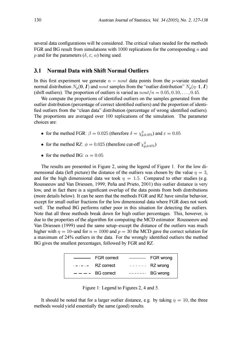
130 Austrian Journal of Statistics,Vol.34(2005),No.2,127-138 several data configurations will be considered.The critical values needed for the methods FGR and BG result from simulations with 1000 replications for the corresponding n and p and for the parameters(,e;a)being used. 3.1 Normal Data with Shift Normal Outliers In this first experiment we generate n-nout data points from the p-variate standard normal distribution N.(0,I)and nout samples from the "outlier distribution"Np(n.1,I) (shift outliers).The proportion of outliers is varied as nout/n =0.05,0.10,...,0.45. We compute the proportions of identified outliers on the samples generated from the outlier distribution(percentage of correct identified outliers)and the proportion of identi- fied outliers from the "clean data"distribution(percentage of wrong identified outliers). The proportions are averaged over 100 replications of the simulation.The parameter choices are: .for the method FGR:B=0.025(therefore =x2.0.97)and =0.05 for the method RZ:=0.025(therefore cut-offx) for the method BG:a =0.05 The results are presented in Figure 2,using the legend of Figure 1.For the low di- mensional data(left picture)the distance of the outliers was chosen by the value n=3, and for the high dimensional data we took n 1.5.Compared to other studies (e.g. Rousseeuw and Van Driessen,1999;Pena and Prieto,2001)this outlier distance is very low,and in fact there is a significant overlap of the data points from both distributions (more details below).It can be seen that the methods FGR and RZ have similar behavior, except for small outlier fractions for the low dimensional data where FGR does not work well.The method BG performs rather poor in this situation for detecting the outliers. Note that all three methods break down for high outlier percentages.This,however,is due to the properties of the algorithm for computing the MCD estimator:Rousseeuw and Van Driessen(1999)used the same setup-except the distance of the outliers was much higher with n=10-and for n =1000 and p=30 the MCD gave the correct solution for a maximum of 24%outliers in the data.For the wrongly identified outliers the method BG gives the smallest percentages,followed by FGR and RZ. FGR correct FGR wrong RZ correct RZ wrong BG correct BG wrong Figure 1:Legend to Figures 2,4 and 5. It should be noted that for a larger outlier distance,e.g.by taking n=10,the three methods would yield essentially the same(good)results.130 Austrian Journal of Statistics, Vol. 34 (2005), No. 2, 127-138 several data configurations will be considered. The critical values needed for the methods FGR and BG result from simulations with 1000 replications for the corresponding n and p and for the parameters (δ, ε; α) being used. 3.1 Normal Data with Shift Normal Outliers In this first experiment we generate n − nout data points from the p-variate standard normal distribution Np(0, I) and nout samples from the “outlier distribution” Np(η ·1, I) (shift outliers). The proportion of outliers is varied as nout/n = 0.05, 0.10, . . . , 0.45. We compute the proportions of identified outliers on the samples generated from the outlier distribution (percentage of correct identified outliers) and the proportion of identi- fied outliers from the “clean data” distribution (percentage of wrong identified outliers). The proportions are averaged over 100 replications of the simulation. The parameter choices are: • for the method FGR: β = 0.025 (therefore δ = χ 2 p,0.975) and ε = 0.05 • for the method RZ: φ = 0.025 (therefore cut-off χ 2 p,0.975) • for the method BG: α = 0.05 The results are presented in Figure 2, using the legend of Figure 1. For the low di￾mensional data (left picture) the distance of the outliers was chosen by the value η = 3, and for the high dimensional data we took η = 1.5. Compared to other studies (e.g. Rousseeuw and Van Driessen, 1999; Pena and Prieto, 2001) this outlier distance is very ˜ low, and in fact there is a significant overlap of the data points from both distributions (more details below). It can be seen that the methods FGR and RZ have similar behavior, except for small outlier fractions for the low dimensional data where FGR does not work well. The method BG performs rather poor in this situation for detecting the outliers. Note that all three methods break down for high outlier percentages. This, however, is due to the properties of the algorithm for computing the MCD estimator: Rousseeuw and Van Driessen (1999) used the same setup–except the distance of the outliers was much higher with η = 10–and for n = 1000 and p = 30 the MCD gave the correct solution for a maximum of 24% outliers in the data. For the wrongly identified outliers the method BG gives the smallest percentages, followed by FGR and RZ. FGR correct FGR wrong RZ correct RZ wrong BG correct BG wrong Figure 1: Legend to Figures 2, 4 and 5. It should be noted that for a larger outlier distance, e.g. by taking η = 10, the three methods would yield essentially the same (good) results