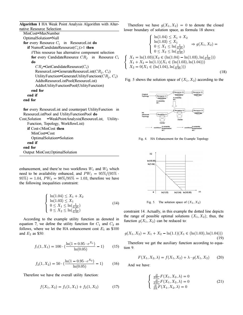
Algorithm 1 HA Weak Point Analysis Algorithm with Alter- Therefore we have g(X1,X2)=0 to denote the closed native Resource Selection lower boundary of solution space,as formula 18 shows: MinCost=MaxNumber OptimalSolution=Null ln(1.04)≤X1+X2 for every Resource Ci in ResourceList do n(1.03)≤X1 0≤X1≤ln(o）) 1 →g(X1,X2)= if NumofCandidateResource(C;)>I then //This resource has alternative component selection 0≤X2≤ln(o.9) for every CandidateResource CRj in Resource Ci X1=ln(1.03)(X2∈(m(1.04)-ln(1.03),ln(o.s)》 do X1+X2-n(1.1)(X1∈(n(1.03),n(1.04)) CR;=GetCandidateResource(Ci) X2=0(X1∈(n(1.04),ln(o)) ResourceList=GenerateResourceList(CRj,Ci) (18) UtilityFunction=GenerateUtilityFunction(CRj,C) AddtoResourceListPool(ResourceList) Fig.5 shows the solution space of (X1,X2)according to the AddtoUtilityFunctionPool(UtilityFunction) end for 取iou6c时 end if end for for every ResourceList and counterpart UtilityFunction in R5rG2 -R5rcC3 ResourceListPool and UtilityFunctionPool do Cost Solution =WeakPointAnalysis(ResourceList,Utility- Function,Topology,WorkflowList) if Cost<MinCost then MinCost=Cost OptimalSolution=Solution Fig.4.HA Enhancement for the Example Topology end if end for Output MinCost,OptimalSolution n10.5 lh(1.04 enhancement,and there're two workflows Wi and W2 which need to be availability enhanced,and PW1 95%/(95%. 95%)=1.04,PW2 =98%/95%=1.03,therefore we have the following inequalities constraint: n1.03 In(1.04)In(10.95)X1 1n(1.04)≤X1+X2 1n(1.03)<X1 0X(p) (14) Fig.5.The solution space of (X1,X2) 0≤X2≤n(o.】 constraint 14.Actually,in this example the dotted line depicts the range of possible optimal solutions (X1,X2);thus,the According to the example utility function as denoted in function g(X1,X2)can be reduced to: equation 7,we define the utility function for Cl and C2 as follows,where we let the HA enhancement cost E as $100 and E2 as $50 g(X1,X2)=X1+X2-ln(1.1)(X1∈(n(1.03),1n(1.04) (19) (1-0.95·e .-1) Therefore we get the auxiliary function according to equa- f1(1,X1)=100.( (15) 1m(0.05) tion 9. F(X1,X2,)=fX1,X2)+入·g(X1,X2) (20) f24,X2)=50-1-0.o5.e）-1） (16) 1n(0.05） And we have: Therefore we have the overall utility function: 化2，-0 F(X,X2,A)=0 (21) f(X1,X2)=f(1,X1)+f2(1,X2) (17) 品F(X1,X2,)=0Algorithm 1 HA Weak Point Analysis Algorithm with Alter￾native Resource Selection MinCost=MaxNumber OptimalSolution=Null for every Resource Ci in ResourceList do if NumofCandidateResource(Ci)>1 then //This resource has alternative component selection for every CandidateResource CRj in Resource Ci do CRj=GetCandidateResource(Ci) ResourceList=GenerateResourceList(CRj , Ci) UtilityFunction=GenerateUtilityFunction(CRj , Ci) AddtoResourceListPool(ResourceList) AddtoUtilityFunctionPool(UtilityFunction) end for end if end for for every ResourceList and counterpart UtilityFunction in ResourceListPool and UtilityFunctionPool do Cost,Solution =WeakPointAnalysis(ResourceList, Utility￾Function, Topology, WorkflowList) if Cost<MinCost then MinCost=Cost OptimalSolution=Solution end if end for Output MinCost,OptimalSolution enhancement, and there’re two workflows W1 and W2 which need to be availability enhanced, and PW1 = 95%/(95% · 95%) = 1.04, PW2 = 98%/95% = 1.03, therefore we have the following inequalities constraint:    ln(1.04) ≤ X1 + X2 ln(1.03) ≤ X1 0 ≤ X1 ≤ ln( 1 0.95 ) 0 ≤ X2 ≤ ln( 1 0.95 ) (14) According to the example utility function as denoted in equation 7, we define the utility function for C1 and C2 as follows, where we let the HA enhancement cost E1 as $100 and E2 as $50: f1(1, X1) = 100 · ( ln(1 − 0.95 · e X1 ) ln(0.05) − 1) (15) f2(1, X2) = 50 · ( ln(1 − 0.95 · e X2 ) ln(0.05) − 1) (16) Therefore we have the overall utility function: f(X1, X2) = f1(1, X1) + f2(1, X2) (17) Therefore we have g(X1, X2) = 0 to denote the closed lower boundary of solution space, as formula 18 shows:    ln(1.04) ≤ X1 + X2 ln(1.03) ≤ X1 0 ≤ X1 ≤ ln( 1 0.95 ) 0 ≤ X2 ≤ ln( 1 0.95 ) ⇒ g(X1, X2) =    X1 = ln(1.03)(X2 ∈ (ln(1.04) − ln(1.03), ln( 1 0.95 ))) X1 + X2 − ln(1.1)(X1 ∈ (ln(1.03), ln(1.04))) X2 = 0(X1 ∈ (ln(1.04), ln( 1 0.95 ))) (18) Fig. 5 shows the solution space of (X1, X2) according to the Fig. 4. HA Enhancement for the Example Topology Fig. 5. The solution space of (X1, X2) constraint 14. Actually, in this example the dotted line depicts the range of possible optimal solutions (X1, X2); thus, the function g(X1, X2) can be reduced to: g(X1, X2) = X1 + X2 − ln(1.1)(X1 ∈ (ln(1.03), ln(1.04))) (19) Therefore we get the auxiliary function according to equa￾tion 9. F(X1, X2, λ) = f(X1, X2) + λ · g(X1, X2) (20) And we have:    ∂ ∂X1 F(X1, X2, λ) = 0 ∂ ∂X2 F(X1, X2, λ) = 0 ∂ ∂λ F(X1, X2, λ) = 0 (21)