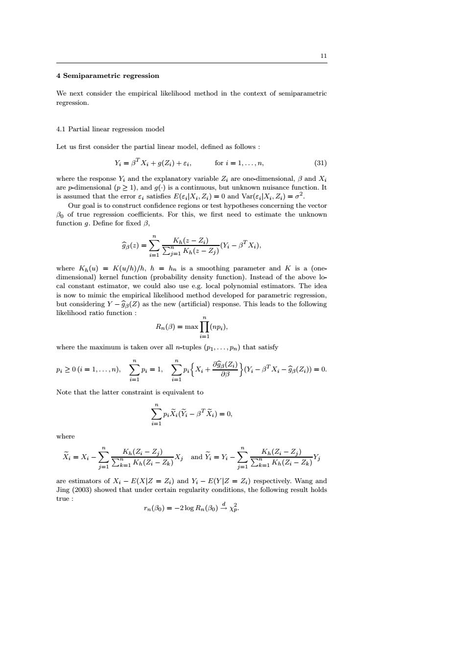
11 4 Semiparametric regression We next consider the empirical likelihood method in the context of semiparametric regression. 4.1 Partial linear regression model Let us first consider the partial linear model,defined as follows Yi=BXi+g(Zi)+ei, for i=1,...,n, (31) where the response Yi and the explanatory variable Zi are one-dimensional,B and Xi are p-dimensional(p 1),and g()is a continuous,but unknown nuisance function.It is assumed that the error ei satisfies E(eilXi,Zi)=0 and Var(eiXi,Zi)=a2 Our goal is to construct confidence regions or test hypotheses concerning the vector Bo of true regression coefficients.For this,we first need to estimate the unknown function g.Define for fixed B. 三- ga()= where Kh(u)=K(u/h)/h,h hn is a smoothing parameter and K is a (one- dimensional)kernel function (probability density function).Instead of the above lo- cal constant estimator,we could also use e.g.local polynomial estimators.The idea is now to mimic the empirical likelihood method developed for parametric regression but considering Y-ge(Z)as the new (artificial)response.This leads to the following likelihood ratio function Rn()=maxp) =1 where the maximum is taken over all n-tuples (p1,...,Pn)that satisfy p≥0(i=1,,n, =1 三nx+西}-x-训-a Note that the latter constraint is equivalent to 三n所-产0-0 where x=X-∑ Kh(Zi-Zj) Kh(Zi-Zj) 名a1K(G-石 are estimators of Xi-E(XZ=Zi)and Yi-E(YIZ=Zi)respectively.Wang and Jing(2003)showed that under certain regularity conditions,the following result holds true: rn(Bo)=-2log Rn(8).11 4 Semiparametric regression We next consider the empirical likelihood method in the context of semiparametric regression. 4.1 Partial linear regression model Let us first consider the partial linear model, defined as follows : Yi = β T Xi + g(Zi) + εi , for i = 1, . . . , n, (31) where the response Yi and the explanatory variable Zi are one-dimensional, β and Xi are p-dimensional (p ≥ 1), and g(·) is a continuous, but unknown nuisance function. It is assumed that the error εi satisfies E(εi |Xi , Zi) = 0 and Var(εi |Xi , Zi) = σ 2 . Our goal is to construct confidence regions or test hypotheses concerning the vector β0 of true regression coefficients. For this, we first need to estimate the unknown function g. Define for fixed β, bgβ(z) = Xn i=1 Kh(z − Zi) Pn j=1 Kh(z − Zj ) (Yi − β T Xi), where Kh(u) = K(u/h)/h, h = hn is a smoothing parameter and K is a (one￾dimensional) kernel function (probability density function). Instead of the above lo￾cal constant estimator, we could also use e.g. local polynomial estimators. The idea is now to mimic the empirical likelihood method developed for parametric regression, but considering Y − bgβ(Z) as the new (artificial) response. This leads to the following likelihood ratio function : Rn(β) = maxYn i=1 (npi), where the maximum is taken over all n-tuples (p1, . . . , pn) that satisfy pi ≥ 0 (i = 1, . . . , n), Xn i=1 pi = 1, Xn i=1 pi n Xi + ∂bgβ(Zi) ∂β o (Yi − β T Xi − bgβ(Zi)) = 0. Note that the latter constraint is equivalent to Xn i=1 piXei(Yei − β T Xei) = 0, where Xei = Xi − Xn j=1 Kh(Zi − Zj ) Pn k=1 Kh(Zi − Zk) Xj and Yei = Yi − Xn j=1 Kh(Zi − Zj ) Pn k=1 Kh(Zi − Zk) Yj are estimators of Xi − E(X|Z = Zi) and Yi − E(Y |Z = Zi) respectively. Wang and Jing (2003) showed that under certain regularity conditions, the following result holds true : rn(β0) = −2 log Rn(β0) d→ χ 2 p