正在加载图片...

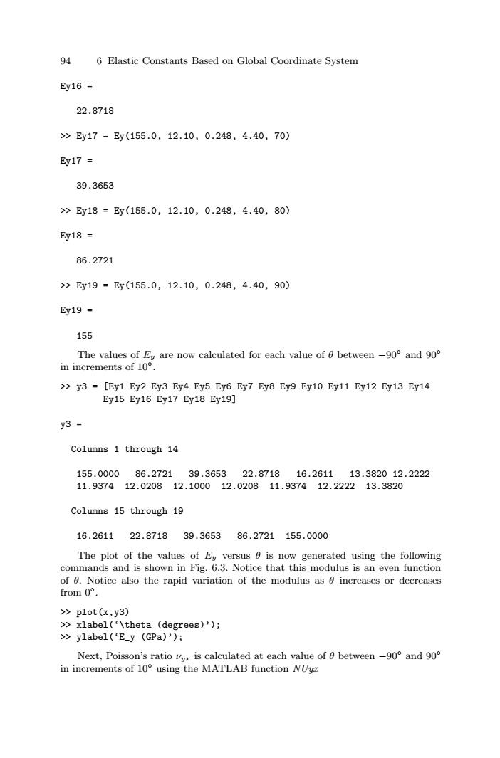
94 6 Elastic Constants Based on Global Coordinate System Ey16= 22.8718 >>Ey17=Ey(155.0,12.10,0.248,4.40,70) Ey17= 39.3653 >Ey18=Ey(155.0,12.10,0.248,4.40,80) Ey18= 86.2721 >Ey19=Ey(155.0,12.10,0.248,4.40,90) Ey19= 155 The values of Ey are now calculated for each value of 0 between-90 and 90 in increments of10° >y3=[Ey1 Ey2 Ey3 Ey4 Ey5 Ey6 Ey7 Ey8 Ey9 Ey10 Ey11 Ey12 Ey13 Ey14 Ey15 Ey16 Ey17 Ey18 Ey19] y3= Columns 1 through 14 155.000086.272139.365322.871816.261113.382012.2222 11.937412.020812.100012.020811.937412.222213.3820 Columns 15 through 19 16.261122.871839.365386.2721155.0000 The plot of the values of Ey versus 0 is now generated using the following commands and is shown in Fig.6.3.Notice that this modulus is an even function of 0.Notice also the rapid variation of the modulus as 0 increases or decreases from0°. >plot(x,y3) >xlabel('\theta (degrees)'); >ylabel('E_y (GPa)'); Next,Poisson's ratio vur is calculated at each value of 0 between -90 and 90 in increments of 10 using the MATLAB function NUyr94 6 Elastic Constants Based on Global Coordinate System Ey16 = 22.8718 >> Ey17 = Ey(155.0, 12.10, 0.248, 4.40, 70) Ey17 = 39.3653 >> Ey18 = Ey(155.0, 12.10, 0.248, 4.40, 80) Ey18 = 86.2721 >> Ey19 = Ey(155.0, 12.10, 0.248, 4.40, 90) Ey19 = 155 The values of Ey are now calculated for each value of θ between −90◦ and 90◦ in increments of 10◦. >> y3 = [Ey1 Ey2 Ey3 Ey4 Ey5 Ey6 Ey7 Ey8 Ey9 Ey10 Ey11 Ey12 Ey13 Ey14 Ey15 Ey16 Ey17 Ey18 Ey19] y3 = Columns 1 through 14 155.0000 86.2721 39.3653 22.8718 16.2611 13.3820 12.2222 11.9374 12.0208 12.1000 12.0208 11.9374 12.2222 13.3820 Columns 15 through 19 16.2611 22.8718 39.3653 86.2721 155.0000 The plot of the values of Ey versus θ is now generated using the following commands and is shown in Fig. 6.3. Notice that this modulus is an even function of θ. Notice also the rapid variation of the modulus as θ increases or decreases from 0◦. >> plot(x,y3) >> xlabel(‘\theta (degrees)’); >> ylabel(‘E_y (GPa)’); Next, Poisson’s ratio νyx is calculated at each value of θ between −90◦ and 90◦ in increments of 10◦ using the MATLAB function NUyx