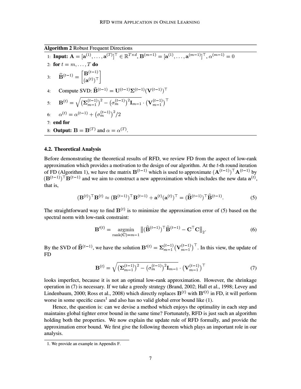
RFD WITH APPLICATION IN ONLINE LEARNING Algorithm 2 Robust Frequent Directions 1:nput:A=a四，..，a(T)]TERTxd,Bm-)=a,.,am-]T,am-=0 2:for t =m,...,T do 3: Bt-1) fB(t-1)7 [(a(D)T Compute SVD:B(t-1)=U(t-1)>(t-1)(V(t-1))T 5: B9=V(②-)2-(-21m-1·(v-)T 6: a国=at-1)+(a-1)2/2 7:end for 8:Output:B=B(T)and aa(T) 4.2.Theoretical Analysis Before demonstrating the theoretical results of RFD,we review FD from the aspect of low-rank approximation which provides a motivation to the design of our algorithm.At the t-th round iteration of FD (Algorithm 1),we have the matrix B(which is used to approximate(A(-1)TA(-1)by (B(-1))TB(-1)and we aim to construct a new approximation which includes the new data a(), that is. (B())TB()(B(-1))TB(-1)+a()(a())T=(B(t-1))TB(-1). (5) The straightforward way to find B()is to minimize the approximation error of(5)based on the spectral norm with low-rank constraint: B()=argmin (B(-1))TB(-1)-CTCll2 (6) rank(C)=m-1 By the SVD of B(1),we have the solution B()V.In this view,the update of FD B©=V(=)2-(o乐-)21m-1·(V-) (7) looks imperfect,because it is not an optimal low-rank approximation.However,the shrinkage operation in(7)is necessary.If we take a greedy strategy (Brand,2002;Hall et al.,1998;Levey and Lindenbaum,2000;Ross et al.,2008)which directly replaces B()with B()in FD,it will perform worse in some specific cases'and also has no valid global error bound like (1). Hence,the question is:can we devise a method which enjoys the optimality in each step and maintains global tighter error bound in the same time?Fortunately,RFD is just such an algorithm holding both the properties.We now explain the update rule of RFD formally,and provide the approximation error bound.We first give the following theorem which plays an important role in our analysis. 1.We provide an example in Appendix F. 7RFD WITH APPLICATION IN ONLINE LEARNING Algorithm 2 Robust Frequent Directions 1: Input: A = [a (1) , . . . , a (T) ] > ∈ R T ×d , B(m−1) = [a (1) , . . . , a (m−1)] >, α (m−1) = 0 2: for t = m, . . . , T do 3: Bb(t−1) =  B(t−1) (a (t) ) >  4: Compute SVD: Bb(t−1) = U(t−1)Σ(t−1)(V(t−1)) > 5: B(t) = q￾ Σ (t−1) m−1
2 − ￾ σ (t−1) m
2 Im−1 · ￾ V (t−1) m−1
> 6: α (t) = α (t−1) + ￾ σ (t−1) m
2 /2 7: end for 8: Output: B = B(T) and α = α (T) . 4.2. Theoretical Analysis Before demonstrating the theoretical results of RFD, we review FD from the aspect of low-rank approximation which provides a motivation to the design of our algorithm. At the t-th round iteration of FD (Algorithm 1), we have the matrix B(t−1) which is used to approximate (A(t−1)) >A(t−1) by (B(t−1)) >B(t−1) and we aim to construct a new approximation which includes the new data a (t) , that is, (B (t) ) >B (t) ≈ (B (t−1)) >B (t−1) + a (t) (a (t) ) > = (Bb(t−1)) >Bb(t−1) . (5) The straightforward way to find B(t) is to minimize the approximation error of (5) based on the spectral norm with low-rank constraint: B 0(t) = argmin rank(C)=m−1 (Bb(t−1)) >Bb(t−1) − C>C 2 . (6) By the SVD of Bb(t−1), we have the solution B0(t) = Σ (t−1) m−1 ￾ V (t−1) m−1
> . In this view, the update of FD B (t) = q￾ Σ (t−1) m−1
2 − ￾ σ (t−1) m
2 Im−1 · ￾ V (t−1) m−1
> (7) looks imperfect, because it is not an optimal low-rank approximation. However, the shrinkage operation in (7) is necessary. If we take a greedy strategy (Brand, 2002; Hall et al., 1998; Levey and Lindenbaum, 2000; Ross et al., 2008) which directly replaces B(t) with B0(t) in FD, it will perform worse in some specific cases1 and also has no valid global error bound like (1). Hence, the question is: can we devise a method which enjoys the optimality in each step and maintains global tighter error bound in the same time? Fortunately, RFD is just such an algorithm holding both the properties. We now explain the update rule of RFD formally, and provide the approximation error bound. We first give the following theorem which plays an important role in our analysis. 1. We provide an example in Appendix F. 7