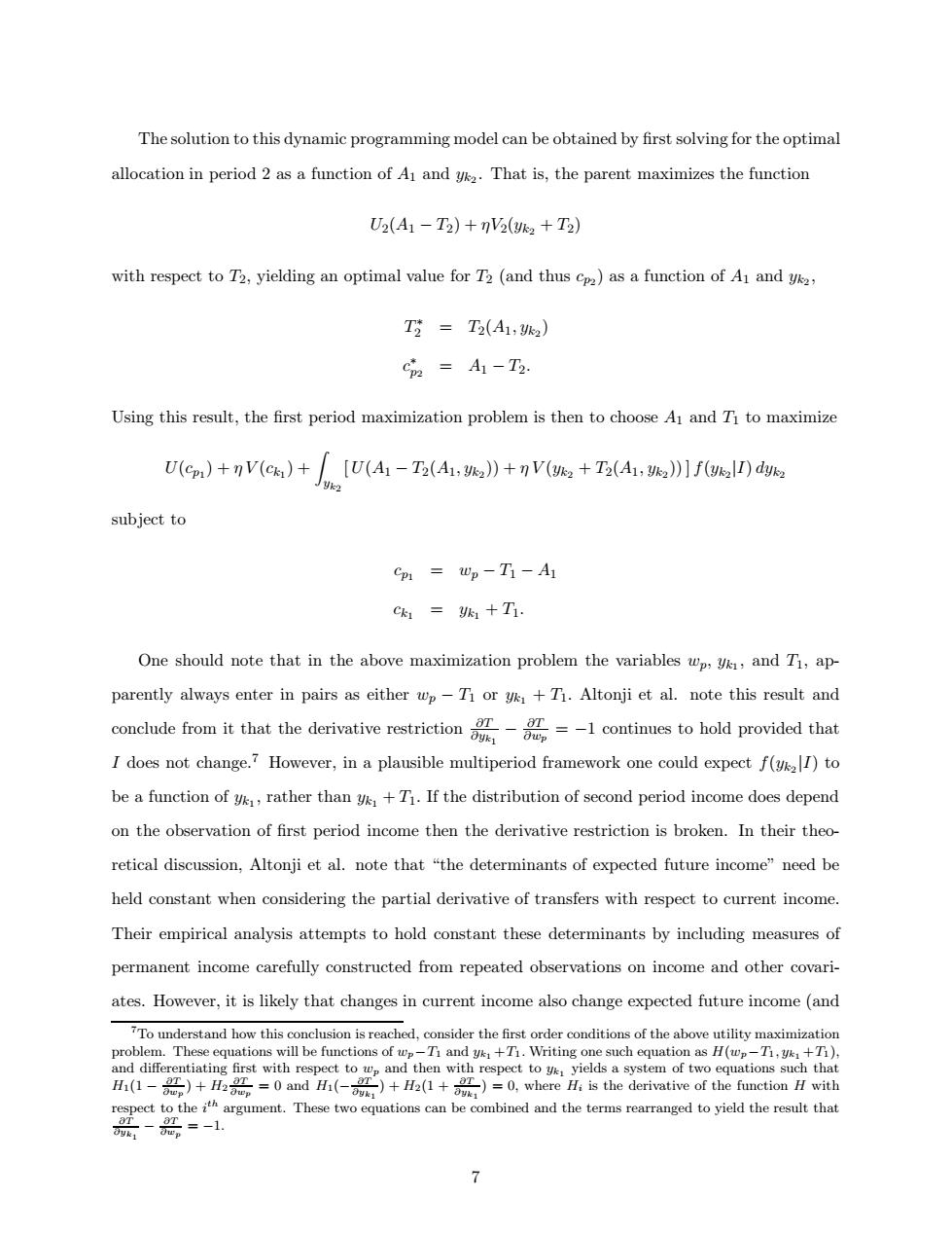
The solution to this dynamic programming model can be obtained by first solving for the optimal allocation in period 2 as a function of A1 and y2.That is,the parent maximizes the function U2(A1-T2)+7V2(y2+T2) with respect to T2,yielding an optimal value for T2(and thus cp2)as a function of A1 and yk2, T2=T2(A1,k2) 2=A-T2. Using this result,the first period maximization problem is then to choose A1 and Ti to maximize U(ep)+nV(ck)+[U(Ai-T2(A1:a))+nV(k2+T2(A1:v))]f(alI)dukz subject to Cp Wp-T1-A1 C%1=1+T1. One should note that in the above maximization problem the variables wp,yk,and T1,ap- parently always enter in pairs as either wp-Ti or y+Ti.Altonji et al.note this result and concde from it that the derivative restriction1contimues to hold provided that I does not change.7 However,in a plausible multiperiod framework one could expect f()to be a function of y,rather than y+T1.If the distribution of second period income does depend on the observation of first period income then the derivative restriction is broken.In their theo- retical discussion,Altonji et al.note that "the determinants of expected future income"need be held constant when considering the partial derivative of transfers with respect to current income. Their empirical analysis attempts to hold constant these determinants by including measures of permanent income carefully constructed from repeated observations on income and other covari- ates.However,it is likely that changes in current income also change expected future income (and 7To understand how this conclusion is reached,consider the first order conditions of the above utility maximization problem.These equations will be functions of wp-Ti and y+Ti.Writing one such equation as H(wp-Ti,y+T), and differentiating first with respect to wp and then with respect to y yields a system of two equations such that (and+H0,where,is the derivative of the function H with respect to the ithargument.These two equations can be combined and the terms rearranged to yield the result that 恶兴=1 7The solution to this dynamic programming model can be obtained by first solving for the optimal allocation in period 2 as a function of A1 and yk2 . That is, the parent maximizes the function U2(A1 − T2) + ηV2(yk2 + T2) with respect to T2, yielding an optimal value for T2 (and thus cp2) as a function of A1 and yk2 , T∗ 2 = T2(A1, yk2) c∗ p2 = A1 − T2. Using this result, the first period maximization problem is then to choose A1 and T1 to maximize U(cp1) + η V (ck1) + yk2 [ U(A1 − T2(A1, yk2)) + η V (yk2 + T2(A1, yk2)) ] f(yk2|I) dyk2 subject to cp1 = wp − T1 − A1 ck1 = yk1 + T1. One should note that in the above maximization problem the variables wp, yk1 , and T1, ap￾parently always enter in pairs as either wp − T1 or yk1 + T1. Altonji et al. note this result and conclude from it that the derivative restriction ∂T ∂yk1 − ∂T ∂wp = −1 continues to hold provided that I does not change.7 However, in a plausible multiperiod framework one could expect f(yk2 |I) to be a function of yk1 , rather than yk1 + T1. If the distribution of second period income does depend on the observation of first period income then the derivative restriction is broken. In their theo￾retical discussion, Altonji et al. note that “the determinants of expected future income” need be held constant when considering the partial derivative of transfers with respect to current income. Their empirical analysis attempts to hold constant these determinants by including measures of permanent income carefully constructed from repeated observations on income and other covari￾ates. However, it is likely that changes in current income also change expected future income (and 7To understand how this conclusion is reached, consider the first order conditions of the above utility maximization problem. These equations will be functions of wp−T1 and yk1 +T1. Writing one such equation as H(wp−T1, yk1 +T1), and differentiating first with respect to wp and then with respect to yk1 yields a system of two equations such that H1(1 − ∂T ∂wp ) + H2 ∂T ∂wp = 0 and H1(− ∂T ∂yk1 ) + H2(1 + ∂T ∂yk1 )=0, where Hi is the derivative of the function H with respect to the i th argument. These two equations can be combined and the terms rearranged to yield the result that ∂T ∂yk1 − ∂T ∂wp = −1. 7