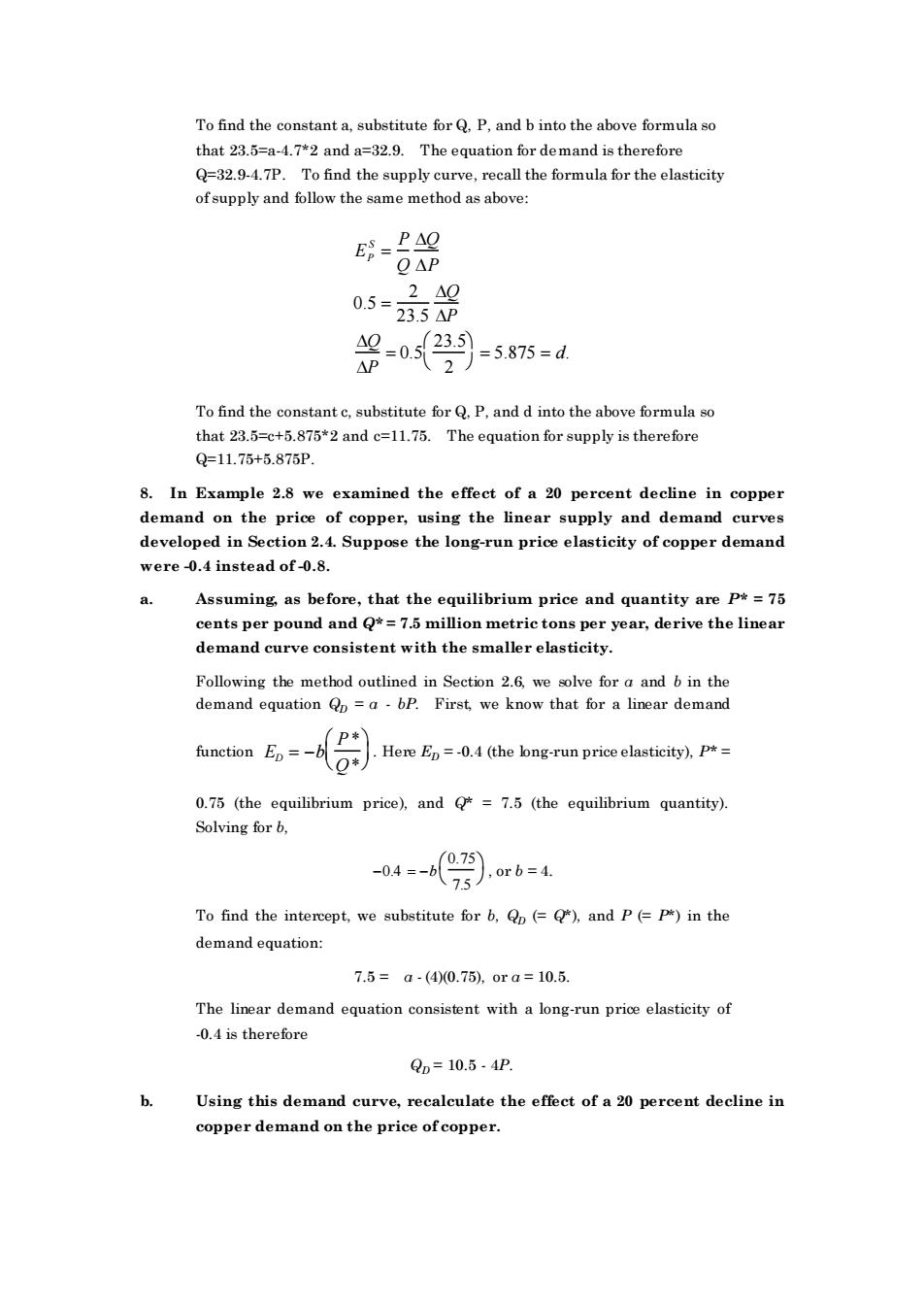
To find the constant a.substitute for Q.P.and b into the above formula so that 23.5=a-4.72 and a=32.9.The equation for demand is therefore Q=32.94.7P To find ofsupply and follow the same method as above: E-PAQ OAP 2△0 0.5=235A =0523 =5.875=d AP 、2 To find the constant c,substitute for Q.P,and d into the above formula so that 23.5=c+5.875*2 and c=11.75.The equation for supply is therefore Q=11.75+5.875P 8.In Example 2.8 we examined the effect of a 2 percent decline in copper demand on the price of copper,using the linear supply and demand curve developed in Section 2.4.Suppose the long-run price elasticity of copper demanc were0.4 instead of-0.8. Assuming,as before,that the equilibrium price and quantity are P*=75 cents per pound and Q*=7.5 million metric tons per year,derive the linear demand curve consistent with the smaller elasticity Following the method outlined in section 2.6 we solve for o nd b in the demand equation=abp First,we know that for a linear demand Here Ep=-0.4(the bng-run price elasticity).P* 0.75 (the equilibrium price),and=7.5 (the equilibrium quantity). Solving forb, -04=-672).orb=4 0.75 To find the intercept,we substitute for b(=),and P(=)in the demandequation: 7.5=a-(40.75,0ra=10.5. The linear demand equation consistent with a long-run price elasticity of -0.4 is therefore Qn=10.5-4P. Using this demand curve,recalculate the effect of a 20 percent decline in copper demand on the price of copper. To find the constant a, substitute for Q, P, and b into the above formula so that 23.5=a-4.7*2 and a=32.9. The equation for demand is therefore Q=32.9-4.7P. To find the supply curve, recall the formula for the elasticity of supply and follow the same method as above:  EP S = P Q Q P 0.5 = 2 23.5 Q P Q P = 0.5 23.5 2     = 5.875 = d. To find the constant c, substitute for Q, P, and d into the above formula so that 23.5=c+5.875*2 and c=11.75. The equation for supply is therefore Q=11.75+5.875P. 8. In Example 2.8 we examined the effect of a 20 percent decline in copper demand on the price of copper, using the linear supply and demand curves developed in Section 2.4. Suppose the long-run price elasticity of copper demand were -0.4 instead of -0.8. a. Assuming, as before, that the equilibrium price and quantity are P* = 75 cents per pound and Q* = 7.5 million metric tons per year, derive the linear demand curve consistent with the smaller elasticity. Following the method outlined in Section 2.6, we solve for a and b in the demand equation QD = a - bP. First, we know that for a linear demand function ED = −b P* Q*       . Here ED = -0.4 (the long-run price elasticity), P* = 0.75 (the equilibrium price), and Q* = 7.5 (the equilibrium quantity). Solving for b, −0.4 = −b 0.75 7.5     , or b = 4. To find the intercept, we substitute for b, QD (= Q*), and P (= P*) in the demand equation: 7.5 = a - (4)(0.75), or a = 10.5. The linear demand equation consistent with a long-run price elasticity of -0.4 is therefore QD = 10.5 - 4P. b. Using this demand curve, recalculate the effect of a 20 percent decline in copper demand on the price of copper