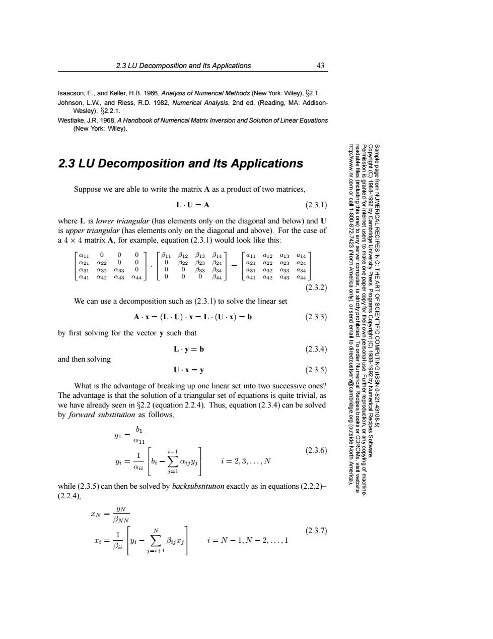
2.3 LU Decomposition and Its Applications 43 Isaacson,E.,and Keller,H.B.1966,Analysis of Numerical Methods (New York:Wiley),82.1. Johnson,L.W.,and Riess,R.D.1982,Numerica/Analysis,2nd ed.(Reading,MA:Addison- Wesley),$2.2.1. Westlake,J.R.1968,A Handbook of Numerical Matrix Inversion and Solution of Linear Equations (New York:Wiley). 2.3 LU Decomposition and Its Applications Suppose we are able to write the matrix A as a product of two matrices, 8= L.U=A (2.3.1) where L is lower triangular (has elements only on the diagonal and below)and U is upper triangular (has elements only on the diagonal and above).For the case of a 4 x 4 matrix A,for example,equation(2.3.1)would look like this: 011 0 0 0 311 12 613 B14 [a11 a12 a13 a14 server 2 a21 022 0 0 022 23 24 a21 a22 a23 a24 (Nort a31 a32 a33 0 0 0 334 a31 a32 a33 a34 041 a42 a43 044 0 0 344 a41 a42 a43 a44 America University Press. THE (2.3.2) ART We can use a decomposition such as(2.3.1)to solve the linear set Progra A·x=(LU)x=L·(Ux)=b (2.3.3) OF SCIENTIFIC( by first solving for the vector y such that 61 L·y=b (2.3.4) and then solving U·x=y (2.3.5) COMPUTING (ISBN 188810920 What is the advantage of breaking up one linear set into two successive ones? The advantage is that the solution of a triangular set of equations is quite trivial,as we have already seen in 82.2 (equation 2.2.4).Thus,equation(2.3.4)can be solved by forward substitution as follows, uurggoglrion Numerical Recipes 10-621 43106 b1 1= 011 (outside i- (2.3.6) North Software. = bi i=2,3,,N j=1 while(2.3.5)can then be solved by backsubstitution exactly as in equations(2.2.2)- (2.2.4), yN TN= BNN (2.3.7) i= i=N-1,N-2,,1 Bu2.3 LU Decomposition and Its Applications 43 Permission is granted for internet users to make one paper copy for their own personal use. Further reproduction, or any copyin Copyright (C) 1988-1992 by Cambridge University Press. Programs Copyright (C) 1988-1992 by Numerical Recipes Software. Sample page from NUMERICAL RECIPES IN C: THE ART OF SCIENTIFIC COMPUTING (ISBN 0-521-43108-5) g of machine￾readable files (including this one) to any server computer, is strictly prohibited. To order Numerical Recipes books or CDROMs, visit website http://www.nr.com or call 1-800-872-7423 (North America only), or send email to directcustserv@cambridge.org (outside North America). Isaacson, E., and Keller, H.B. 1966, Analysis of Numerical Methods (New York: Wiley), §2.1. Johnson, L.W., and Riess, R.D. 1982, Numerical Analysis, 2nd ed. (Reading, MA: Addison￾Wesley), §2.2.1. Westlake, J.R. 1968, A Handbook of Numerical Matrix Inversion and Solution of Linear Equations (New York: Wiley). 2.3 LU Decomposition and Its Applications Suppose we are able to write the matrix A as a product of two matrices, L · U = A (2.3.1) where L is lower triangular (has elements only on the diagonal and below) and U is upper triangular (has elements only on the diagonal and above). For the case of a 4 × 4 matrix A, for example, equation (2.3.1) would look like this:   α11 000 α21 α22 0 0 α31 α32 α33 0 α41 α42 α43 α44   ·   β11 β12 β13 β14 0 β22 β23 β24 0 0 β33 β34 000 β44   =   a11 a12 a13 a14 a21 a22 a23 a24 a31 a32 a33 a34 a41 a42 a43 a44   (2.3.2) We can use a decomposition such as (2.3.1) to solve the linear set A · x = (L · U) · x = L · (U · x) = b (2.3.3) by first solving for the vector y such that L · y = b (2.3.4) and then solving U · x = y (2.3.5) What is the advantage of breaking up one linear set into two successive ones? The advantage is that the solution of a triangular set of equations is quite trivial, as we have already seen in §2.2 (equation 2.2.4). Thus, equation (2.3.4) can be solved by forward substitution as follows, y1 = b1 α11 yi = 1 αii  bi − i−1 j=1 αijyj   i = 2, 3,...,N (2.3.6) while (2.3.5) can then be solved by backsubstitution exactly as in equations (2.2.2)– (2.2.4), xN = yN βNN xi = 1 βii  yi −  N j=i+1 βijxj   i = N − 1, N − 2,..., 1 (2.3.7)