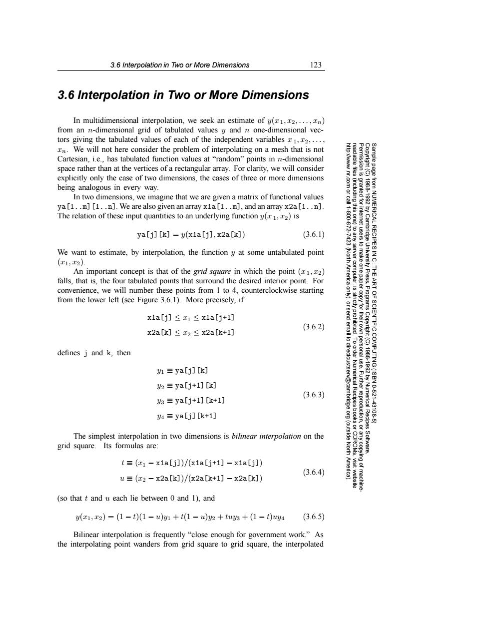
3.6 Interpolation in Two or More Dimensions 123 3.6 Interpolation in Two or More Dimensions In multidimensional interpolation,we seek an estimate of y(1,2,...,n) from an n-dimensional grid of tabulated values y and n one-dimensional vec- tors giving the tabulated values of each of the independent variables 1,2,..., n.We will not here consider the problem of interpolating on a mesh that is not Cartesian,i.e.,has tabulated function values at"random"points in n-dimensional space rather than at the vertices of a rectangular array.For clarity,we will consider explicitly only the case of two dimensions,the cases of three or more dimensions being analogous in every way. In two dimensions,we imagine that we are given a matrix of functional values 98 鱼君 ya [1..m][1..n].We are also given an array xia[1..m],and an array x2a[1..n]. The relation of these input quantities to an underlying function y(1,2)is ya[j][k]=y(x1a[j],x2a[k]) (3.6.1) RECIPESI We want to estimate,by interpolation,the function y at some untabulated point (T1,T2) An important concept is that of the grid square in which the point(1,x2) falls,that is,the four tabulated points that surround the desired interior point.For convenience,we will number these points from I to 4,counterclockwise starting from the lower left(see Figure 3.6.1).More precisely,if 9 x1a[j]≤x1≤x1a[j+1] (3.6.2) OF SCIENTIFIC( x2a[k]≤x2≤x2a[k+1] defines j and k,then y1≡ya[j][k] (ISBN 2≡ya[j+1][k] (3.6.3) 3≡ya[j+1][k+1] Numerica 10.621 y4≡ya[j][k+1] 39 43108 (outside Recipes The simplest interpolation in two dimensions is bilinear interpolation on the grid square.Its formulas are: North t≡(x1-x1a[j])/(x1a[j+1]-x1a[j]) (3.6.4) u≡(r2-x2a[k])/(x2a[k+1]-x2a[x]) (so that t and u each lie between 0 and 1).and (x1,x2)=(1-t)(1-u)班1+t(1-u)2+tug+(1-t)uy4 (3.6.5) Bilinear interpolation is frequently "close enough for government work."As the interpolating point wanders from grid square to grid square,the interpolated3.6 Interpolation in Two or More Dimensions 123 Permission is granted for internet users to make one paper copy for their own personal use. Further reproduction, or any copyin Copyright (C) 1988-1992 by Cambridge University Press. Programs Copyright (C) 1988-1992 by Numerical Recipes Software. Sample page from NUMERICAL RECIPES IN C: THE ART OF SCIENTIFIC COMPUTING (ISBN 0-521-43108-5) g of machine￾readable files (including this one) to any server computer, is strictly prohibited. To order Numerical Recipes books or CDROMs, visit website http://www.nr.com or call 1-800-872-7423 (North America only), or send email to directcustserv@cambridge.org (outside North America). 3.6 Interpolation in Two or More Dimensions In multidimensional interpolation, we seek an estimate of y(x1, x2,...,xn) from an n-dimensional grid of tabulated values y and n one-dimensional vec￾tors giving the tabulated values of each of the independent variables x 1, x2,..., xn. We will not here consider the problem of interpolating on a mesh that is not Cartesian, i.e., has tabulated function values at “random” points in n-dimensional space rather than at the vertices of a rectangular array. For clarity, we will consider explicitly only the case of two dimensions, the cases of three or more dimensions being analogous in every way. In two dimensions, we imagine that we are given a matrix of functional values ya[1..m][1..n]. We are also given an array x1a[1..m], and an array x2a[1..n]. The relation of these input quantities to an underlying function y(x 1, x2) is ya[j][k] = y(x1a[j], x2a[k]) (3.6.1) We want to estimate, by interpolation, the function y at some untabulated point (x1, x2). An important concept is that of the grid square in which the point (x1, x2) falls, that is, the four tabulated points that surround the desired interior point. For convenience, we will number these points from 1 to 4, counterclockwise starting from the lower left (see Figure 3.6.1). More precisely, if x1a[j] ≤ x1 ≤ x1a[j+1] x2a[k] ≤ x2 ≤ x2a[k+1] (3.6.2) defines j and k, then y1 ≡ ya[j][k] y2 ≡ ya[j+1][k] y3 ≡ ya[j+1][k+1] y4 ≡ ya[j][k+1] (3.6.3) The simplest interpolation in two dimensions is bilinear interpolation on the grid square. Its formulas are: t ≡ (x1 − x1a[j])/(x1a[j+1] − x1a[j]) u ≡ (x2 − x2a[k])/(x2a[k+1] − x2a[k]) (3.6.4) (so that t and u each lie between 0 and 1), and y(x1, x2) = (1 − t)(1 − u)y1 + t(1 − u)y2 + tuy3 + (1 − t)uy4 (3.6.5) Bilinear interpolation is frequently “close enough for government work.” As the interpolating point wanders from grid square to grid square, the interpolated