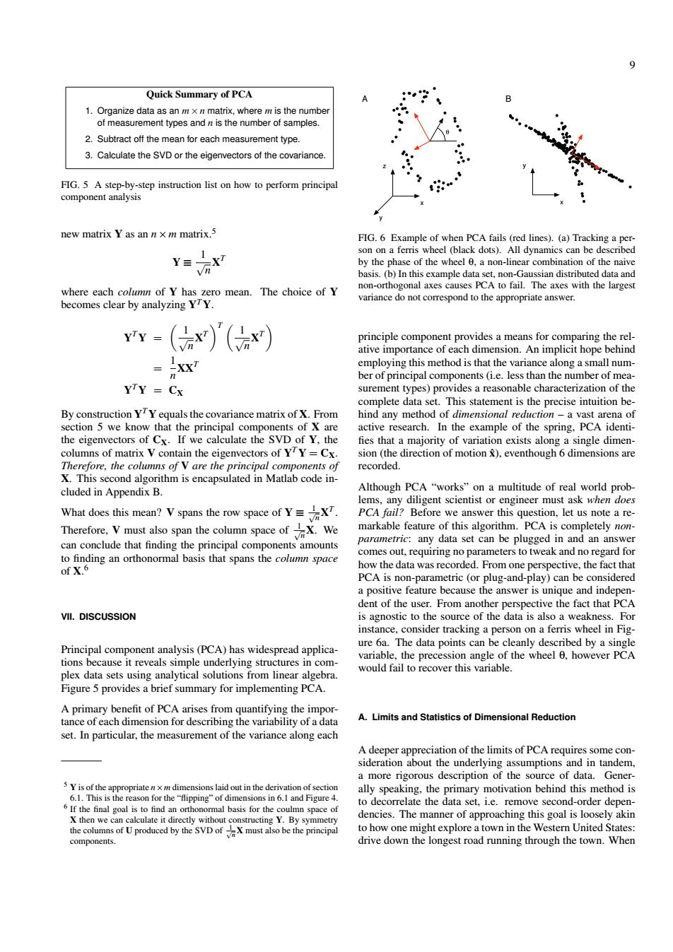
Quick Summary of PCA 1.Organize data as an m x n matrix,where m is the number of measurement types and n is the number of samples. 2.Subtract off the mean for each measurement type. 3.Calculate the SVD or the eigenvectors of the covariance. FIG.5 A step-by-step instruction list on how to perform principal component analysis new matrix Y as an n x m matrix.5 FIG.6 Example of when PCA fails (red lines).(a)Tracking a per- 1 son on a ferris wheel (black dots).All dynamics can be described by the phase of the wheel 0.a non-linear combination of the naive Vn basis.(b)In this example data set,non-Gaussian distributed data and non-orthogonal axes causes PCA to fail.The axes with the largest where each column of Y has zero mean.The choice of Y becomes clear by analyzing YTY. variance do not correspond to the appropriate answer. =(x)'(x principle component provides a means for comparing the rel- ative importance of each dimension.An implicit hope behind x employing this method is that the variance along a small num- ber of principal components(i.e.less than the number of mea- YTY =Cx surement types)provides a reasonable characterization of the complete data set.This statement is the precise intuition be- By construction YTY equals the covariance matrix of X.From hind any method of dimensional reduction-a vast arena of section 5 we know that the principal components of X are active research.In the example of the spring,PCA identi- the eigenvectors of Cx.If we calculate the SVD of Y,the fies that a majority of variation exists along a single dimen- columns of matrix V contain the eigenvectors of YTY=Cx. sion(the direction of motion &)eventhough 6 dimensions are Therefore,the columns of V are the principal components of recorded. X.This second algorithm is encapsulated in Matlab code in- cluded in Appendix B. Although PCA "works"on a multitude of real world prob- lems,any diligent scientist or engineer must ask when does What does this mean?V spans the row space of Y PCA fail?Before we answer this question,let us note a re- Therefore,V must also span the column space of.We markable feature of this algorithm.PCA is completely non- can conclude that finding the principal components amounts parametric:any data set can be plugged in and an answer comes out,requiring no parameters to tweak and no regard for to finding an orthonormal basis that spans the column space of X.6 how the data was recorded.From one perspective,the fact that PCA is non-parametric(or plug-and-play)can be considered a positive feature because the answer is unique and indepen- dent of the user.From another perspective the fact that PCA VIl.DISCUSSION is agnostic to the source of the data is also a weakness.For instance,consider tracking a person on a ferris wheel in Fig- ure 6a.The data points can be cleanly described by a single Principal component analysis(PCA)has widespread applica- tions because it reveals simple underlying structures in com- variable,the precession angle of the wheel 0,however PCA would fail to recover this variable. plex data sets using analytical solutions from linear algebra. Figure 5 provides a brief summary for implementing PCA. A primary benefit of PCA arises from quantifying the impor- tance of each dimension for describing the variability of a data A.Limits and Statistics of Dimensional Reduction set.In particular,the measurement of the variance along each A deeper appreciation of the limits of PCA requires some con- sideration about the underlying assumptions and in tandem, a more rigorous description of the source of data.Gener 5Yis of the appropriatendimensions laid out in the derivation of section ally speaking,the primary motivation behind this method is 6.1.This is the reason for the "flipping"of dimensions in 6.1 and Figure 4. 6 If the final goal is to find an orthonormal basis for the coulmn space of to decorrelate the data set,i.e.remove second-order depen- X then we can calculate it directly without constructing Y.By symmetry dencies.The manner of approaching this goal is loosely akin the columns of U produced by the SVD ofX must also be the principal to how one might explore a town in the Western United States: components. drive down the longest road running through the town.When9 Quick Summary of PCA 1. Organize data as an m×n matrix, where m is the number of measurement types and n is the number of samples. 2. Subtract off the mean for each measurement type. 3. Calculate the SVD or the eigenvectors of the covariance. FIG. 5 A step-by-step instruction list on how to perform principal component analysis new matrix Y as an n×m matrix.5 Y ≡ 1 √ n X T where each column of Y has zero mean. The choice of Y becomes clear by analyzing Y TY. Y TY =  1 √ n X T T  1 √ n X T  = 1 n XXT Y TY = CX By construction Y TY equals the covariance matrix of X. From section 5 we know that the principal components of X are the eigenvectors of CX. If we calculate the SVD of Y, the columns of matrix V contain the eigenvectors of Y TY = CX. Therefore, the columns of V are the principal components of X. This second algorithm is encapsulated in Matlab code in￾cluded in Appendix B. What does this mean? V spans the row space of Y ≡ √ 1 n X T . Therefore, V must also span the column space of √ 1 n X. We can conclude that finding the principal components amounts to finding an orthonormal basis that spans the column space of X. 6 VII. DISCUSSION Principal component analysis (PCA) has widespread applica￾tions because it reveals simple underlying structures in com￾plex data sets using analytical solutions from linear algebra. Figure 5 provides a brief summary for implementing PCA. A primary benefit of PCA arises from quantifying the impor￾tance of each dimension for describing the variability of a data set. In particular, the measurement of the variance along each 5 Y is of the appropriate n×m dimensions laid out in the derivation of section 6.1. This is the reason for the “flipping” of dimensions in 6.1 and Figure 4. 6 If the final goal is to find an orthonormal basis for the coulmn space of X then we can calculate it directly without constructing Y. By symmetry the columns of U produced by the SVD of √1 n X must also be the principal components. A B x y x y z θ FIG. 6 Example of when PCA fails (red lines). (a) Tracking a per￾son on a ferris wheel (black dots). All dynamics can be described by the phase of the wheel θ, a non-linear combination of the naive basis. (b) In this example data set, non-Gaussian distributed data and non-orthogonal axes causes PCA to fail. The axes with the largest variance do not correspond to the appropriate answer. principle component provides a means for comparing the rel￾ative importance of each dimension. An implicit hope behind employing this method is that the variance along a small num￾ber of principal components (i.e. less than the number of mea￾surement types) provides a reasonable characterization of the complete data set. This statement is the precise intuition be￾hind any method of dimensional reduction – a vast arena of active research. In the example of the spring, PCA identi- fies that a majority of variation exists along a single dimen￾sion (the direction of motion xˆ), eventhough 6 dimensions are recorded. Although PCA “works” on a multitude of real world prob￾lems, any diligent scientist or engineer must ask when does PCA fail? Before we answer this question, let us note a re￾markable feature of this algorithm. PCA is completely non￾parametric: any data set can be plugged in and an answer comes out, requiring no parameters to tweak and no regard for how the data was recorded. From one perspective, the fact that PCA is non-parametric (or plug-and-play) can be considered a positive feature because the answer is unique and indepen￾dent of the user. From another perspective the fact that PCA is agnostic to the source of the data is also a weakness. For instance, consider tracking a person on a ferris wheel in Fig￾ure 6a. The data points can be cleanly described by a single variable, the precession angle of the wheel θ, however PCA would fail to recover this variable. A. Limits and Statistics of Dimensional Reduction A deeper appreciation of the limits of PCA requires some con￾sideration about the underlying assumptions and in tandem, a more rigorous description of the source of data. Gener￾ally speaking, the primary motivation behind this method is to decorrelate the data set, i.e. remove second-order depen￾dencies. The manner of approaching this goal is loosely akin to how one might explore a town in the Western United States: drive down the longest road running through the town. When