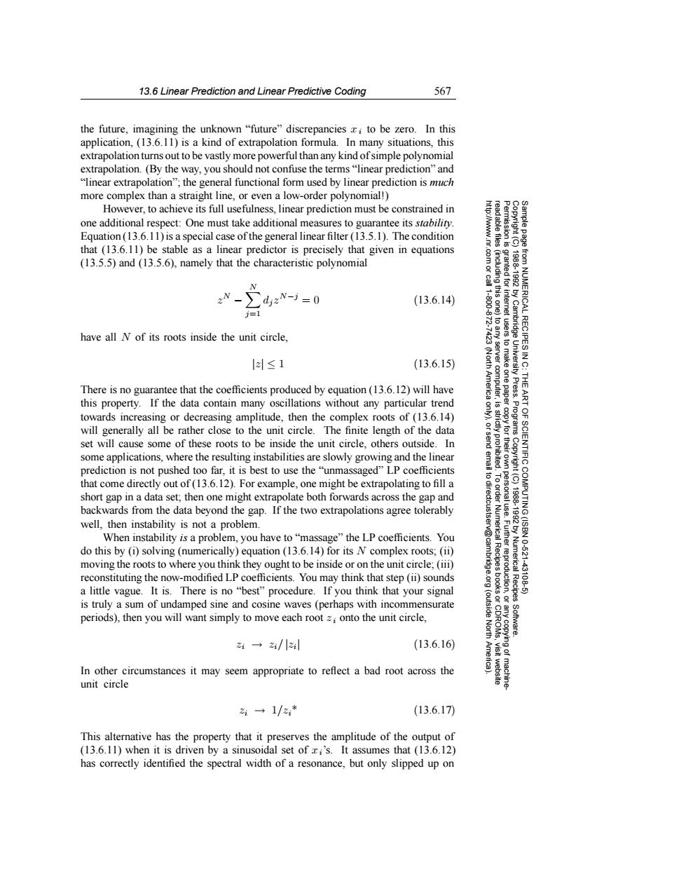
13.6 Linear Prediction and Linear Predictive Coding 567 the future,imagining the unknown"future"discrepancies x;to be zero.In this application,(13.6.11)is a kind of extrapolation formula.In many situations,this extrapolation turns out to be vastly more powerful than any kind of simple polynomial extrapolation.(By the way,you should not confuse the terms"linear prediction"and "linear extrapolation";the general functional form used by linear prediction is much more complex than a straight line,or even a low-order polynomial!) However,to achieve its full usefulness,linear prediction must be constrained in one additional respect:One must take additional measures to guarantee its stability. Equation(13.6.11)is a special case ofthe general linear filter(13.5.1).The condition that(13.6.11)be stable as a linear predictor is precisely that given in equations (13.5.5)and (13.5.6),namely that the characteristic polynomial 思2君 81 N >dzN-3=0 (13.6.14) ICAL j=1 have all N of its roots inside the unit circle. |z≤1 (13.6.15) 9 There is no guarantee that the coefficients produced by equation(13.6.12)will have 2人 this property.If the data contain many oscillations without any particular trend towards increasing or decreasing amplitude,then the complex roots of(13.6.14) will generally all be rather close to the unit circle.The finite length of the data gO 9 set will cause some of these roots to be inside the unit circle.others outside.In some applications,where the resulting instabilities are slowly growing and the linear prediction is not pushed too far,it is best to use the "unmassaged"LP coefficients that come directly out of(13.6.12).For example,one might be extrapolating to fill a 61 short gap in a data set;then one might extrapolate both forwards across the gap and backwards from the data beyond the gap.If the two extrapolations agree tolerably well,then instability is not a problem. When instability is a problem,you have to"massage"the LP coefficients.You do this by (i)solving(numerically)equation(13.6.14)for its N complex roots;(ii) moving the roots to where you think they ought to be inside or on the unit circle;(iii) ©e Numerica 10-521 reconstituting the now-modified LP coefficients.You may think that step (ii)sounds 431 a little vague.It is.There is no"best"procedure.If you think that your signal Recipes is truly a sum of undamped sine and cosine waves(perhaps with incommensurate periods),then you will want simply to move each root z;onto the unit circle. North 2→4/lz (13.6.16) In other circumstances it may seem appropriate to reflect a bad root across the unit circle 2一1/2，* (13.6.17) This alternative has the property that it preserves the amplitude of the output of (13.6.11)when it is driven by a sinusoidal set of zi's.It assumes that (13.6.12) has correctly identified the spectral width of a resonance,but only slipped up on13.6 Linear Prediction and Linear Predictive Coding 567 Permission is granted for internet users to make one paper copy for their own personal use. Further reproduction, or any copyin Copyright (C) 1988-1992 by Cambridge University Press. Programs Copyright (C) 1988-1992 by Numerical Recipes Software. Sample page from NUMERICAL RECIPES IN C: THE ART OF SCIENTIFIC COMPUTING (ISBN 0-521-43108-5) g of machine￾readable files (including this one) to any server computer, is strictly prohibited. To order Numerical Recipes books or CDROMs, visit website http://www.nr.com or call 1-800-872-7423 (North America only), or send email to directcustserv@cambridge.org (outside North America). the future, imagining the unknown “future” discrepancies xi to be zero. In this application, (13.6.11) is a kind of extrapolation formula. In many situations, this extrapolation turns out to be vastly more powerful than any kind of simple polynomial extrapolation. (By the way, you should not confuse the terms “linear prediction” and “linear extrapolation”; the general functional form used by linear prediction is much more complex than a straight line, or even a low-order polynomial!) However, to achieve its full usefulness, linear prediction must be constrained in one additional respect: One must take additional measures to guarantee its stability. Equation (13.6.11) is a special case of the general linear filter (13.5.1). The condition that (13.6.11) be stable as a linear predictor is precisely that given in equations (13.5.5) and (13.5.6), namely that the characteristic polynomial zN −
N j=1 dj zN−j =0 (13.6.14) have all N of its roots inside the unit circle, |z| ≤ 1 (13.6.15) There is no guarantee that the coefficients produced by equation (13.6.12) will have this property. If the data contain many oscillations without any particular trend towards increasing or decreasing amplitude, then the complex roots of (13.6.14) will generally all be rather close to the unit circle. The finite length of the data set will cause some of these roots to be inside the unit circle, others outside. In some applications, where the resulting instabilities are slowly growing and the linear prediction is not pushed too far, it is best to use the “unmassaged” LP coefficients that come directly out of (13.6.12). For example, one might be extrapolating to fill a short gap in a data set; then one might extrapolate both forwards across the gap and backwards from the data beyond the gap. If the two extrapolations agree tolerably well, then instability is not a problem. When instability is a problem, you have to “massage” the LP coefficients. You do this by (i) solving (numerically) equation (13.6.14) for its N complex roots; (ii) moving the roots to where you think they ought to be inside or on the unit circle; (iii) reconstituting the now-modified LP coefficients. You may think that step (ii) sounds a little vague. It is. There is no “best” procedure. If you think that your signal is truly a sum of undamped sine and cosine waves (perhaps with incommensurate periods), then you will want simply to move each root z i onto the unit circle, zi → zi/ |zi| (13.6.16) In other circumstances it may seem appropriate to reflect a bad root across the unit circle zi → 1/zi* (13.6.17) This alternative has the property that it preserves the amplitude of the output of (13.6.11) when it is driven by a sinusoidal set of xi’s. It assumes that (13.6.12) has correctly identified the spectral width of a resonance, but only slipped up on