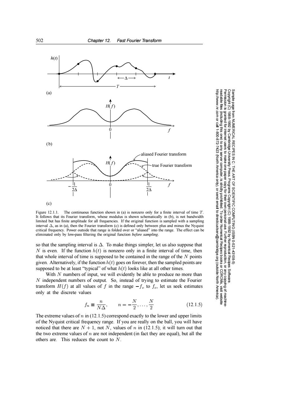
502 Chapter 12.Fast Fourier Transform h(0 (a) H http://www.r. Permission is read able files .com or call granted for (including this one) 19881992 11-800.872 (b) from NUMERICAL RECIPES IN C: /Cambridge aliased Fourier transform true Fourier transform (North America server computer, tusers to make one paper UnN电.t THE ART 2△ strictly proh Programs (c) Figure 12.1.1.The continuous function shown in (a)is nonzero only for a finite interval of time T. It follows that its Fourier transform,whose modulus is shown schematically in(b),is not bandwidth to dir limited but has finite amplitude for all frequencies.If the original function is sampled with a sampling interval A,as in (a),then the Fourier transform (c)is defined only between plus and minus the Nyquist critical frequency.Power outside that range is folded over or "aliased"into the range.The effect can be eliminated only by low-pass filtering the original function before sampling. v@cam so that the sampling interval is A.To make things simpler,let us also suppose that N is even.If the function h(t)is nonzero only in a finite interval of time,then that whole interval of time is supposed to be contained in the range of the N points 乳 1881892 OF SCIENTIFIC COMPUTING(ISBN .Further reproduction, Numerical Recipes 10-621 43108 given.Alternatively,if the function h(t)goes on forever,then the sampled points are supposed to be at least"typical"of what h(t)looks like at all other times. (outside With N numbers of input,we will evidently be able to produce no more than N independent numbers of output.So,instead of trying to estimate the Fourier North Software. transform H(f)at all values of f in the range -fe to fe,let us seek estimates only at the discrete values visit website fn=N△' n=- (12.1.5) machine 292 The extreme values of n in(12.1.5)correspond exactly to the lower and upper limits of the Nyquist critical frequency range.If you are really on the ball,you will have noticed that there are N+1,not N.values of n in (12.1.5):it will turn out that the two extreme values of n are not independent(in fact they are equal),but all the others are.This reduces the count to N.502 Chapter 12. Fast Fourier Transform Permission is granted for internet users to make one paper copy for their own personal use. Further reproduction, or any copyin Copyright (C) 1988-1992 by Cambridge University Press. Programs Copyright (C) 1988-1992 by Numerical Recipes Software. Sample page from NUMERICAL RECIPES IN C: THE ART OF SCIENTIFIC COMPUTING (ISBN 0-521-43108-5) g of machine￾readable files (including this one) to any server computer, is strictly prohibited. To order Numerical Recipes books or CDROMs, visit website http://www.nr.com or call 1-800-872-7423 (North America only), or send email to directcustserv@cambridge.org (outside North America). h(t) t (a) f 0 H( f ) (b) (c) aliased Fourier transform true Fourier transform 0 H( f ) 1 2∆ 1 2∆ − f ∆ T Figure 12.1.1. The continuous function shown in (a) is nonzero only for a finite interval of time T. It follows that its Fourier transform, whose modulus is shown schematically in (b), is not bandwidth limited but has finite amplitude for all frequencies. If the original function is sampled with a sampling interval ∆, as in (a), then the Fourier transform (c) is defined only between plus and minus the Nyquist critical frequency. Power outside that range is folded over or “aliased” into the range. The effect can be eliminated only by low-pass filtering the original function before sampling. so that the sampling interval is ∆. To make things simpler, let us also suppose that N is even. If the function h(t) is nonzero only in a finite interval of time, then that whole interval of time is supposed to be contained in the range of the N points given. Alternatively, if the function h(t) goes on forever, then the sampled points are supposed to be at least “typical” of what h(t) looks like at all other times. With N numbers of input, we will evidently be able to produce no more than N independent numbers of output. So, instead of trying to estimate the Fourier transform H(f) at all values of f in the range −fc to fc, let us seek estimates only at the discrete values fn ≡ n N∆, n = −N 2 ,..., N 2 (12.1.5) The extreme values of n in (12.1.5) correspond exactly to the lower and upper limits of the Nyquist critical frequency range. If you are really on the ball, you will have noticed that there are N + 1, not N, values of n in (12.1.5); it will turn out that the two extreme values of n are not independent (in fact they are equal), but all the others are. This reduces the count to N