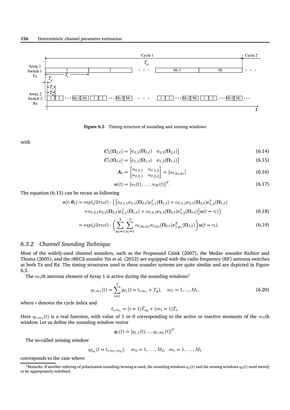
156 Deterministic channel parameter estimation Cyele 1 Cycle 2 2 Mi-l …M网g口…g···☐2…M网a2…网a· Rx Figure 6.5 Timing structure of sounding and sensing windows with C2(2）=【e212c2.22j (6.14 C1(1.）=[c11(1,e）c1.21,] (6.15) (6.16 (9=a(),w(tj7 (6.17刀 The equation(6.13)can be recast as following s(t0)=exp(j2 avit0·{[ae1,1c21(2.)c1(1.d)+a1,2c2,1(2jcH2z(1) +a.21c2.2(2jc.(1)+au2.2c2.2(2.c.2(1.】ut-} (6.18) (6.19y 6.3.2 Channel Sounding Technique both and R.The timing structures used in these sounder systems are quire simlar and are depicred in Figure The mth antennae of Array 1 is active during the sounding windows (6.20) i=1 where i denotes the cycle index and t4m=(位-1)Tg+(m1-1)T. no theorn te m The so-called sensing window 9r(t-t.m.m)2m2=1,,M2,m1=1,,M corresponds to the case where ng is used.the s ndowsand the senin windows)eed merely 156 Deterministic channel parameter estimation 1 Tt 2 M1-1 M1 1 2 M2-1 M2 Cycle 1 Cycle 2 1 2 1 2 1 2 Tg Tsc Tcy t Tr Array 1 Switch 1 Tx Array 2 Switch 2 Rx M2-1 M2 M2-1 M2 M2-1 M2 Figure 6.5 Timing structure of sounding and sensing windows with C2(Ω2,ℓ) = c2,1(Ω2,ℓ) c2,2(Ω2,ℓ) (6.14) C1(Ω1,ℓ) = c1,1(Ω1,ℓ) c1,2(Ω1,ℓ) (6.15) Aℓ =  αℓ,1,1 αℓ,1,2 αℓ,2,1 αℓ,2,2  = [αℓ,p2,p1 ] (6.16) u(t) = [u1(t), . . . , uM(t)]T . (6.17) The equation (6.13) can be recast as following s(t; θℓ) = exp(j2πνℓt) · αℓ,1,1c2,1(Ω2,ℓ)c T 1,1 (Ω1,ℓ) + αℓ,1,2c2,1(Ω2,ℓ)c T 1,2 (Ω1,ℓ) +αℓ,2,1c2,2(Ω2,ℓ)c T 1,1 (Ω1,ℓ) + αℓ,2,2c2,2(Ω2,ℓ)c T 1,2 (Ω1,ℓ) u(t − τℓ) (6.18) = exp(j2πνℓt) · X 2 p2=1 X 2 p1=1 αℓ,p2,p1 c2,p2 (Ω2,ℓ)c T 1,p1 (Ω1,ℓ)  u(t − τℓ). (6.19) 6.3.2 Channel Sounding Technique Most of the widely-used channel sounders, such as the Propsound Czink (2007), the Medav sounder Richter and Thoma (2005), and the rBECS sounder Yin et al. (2012) are equipped with the radio frequency (RF) antenna switches at both Tx and Rx. The timing structures used in these sounder systems are quite similar and are depicted in Figure 6.5. The m1th antenna element of Array 1 is active during the sounding windows1 q1,m1 (t) = X I i=1 qTt (t − ti,m1 + Tg), m1 = 1, ..., M1, (6.20) where i denotes the cycle index and ti,m1 = (i − 1)Tcy + (m1 − 1)Tt. Here q1,m1 (t) is a real function, with value of 1 or 0 corresponding to the active or inactive moments of the m1th window. Let us define the sounding window vector q1(t) .= [q1,1(t), ..., q1,M1 (t)]T . The so-called sensing window qTsc (t − ti,m1,m2 ), m2 = 1, . . . , M2, m1 = 1, . . . , M1 corresponds to the case where 1Remarks: If another ordering of polarization sounding/sensing is used, the sounding windows q1(t) and the sensing windows q2(t) need merely to be appropriately redefined.