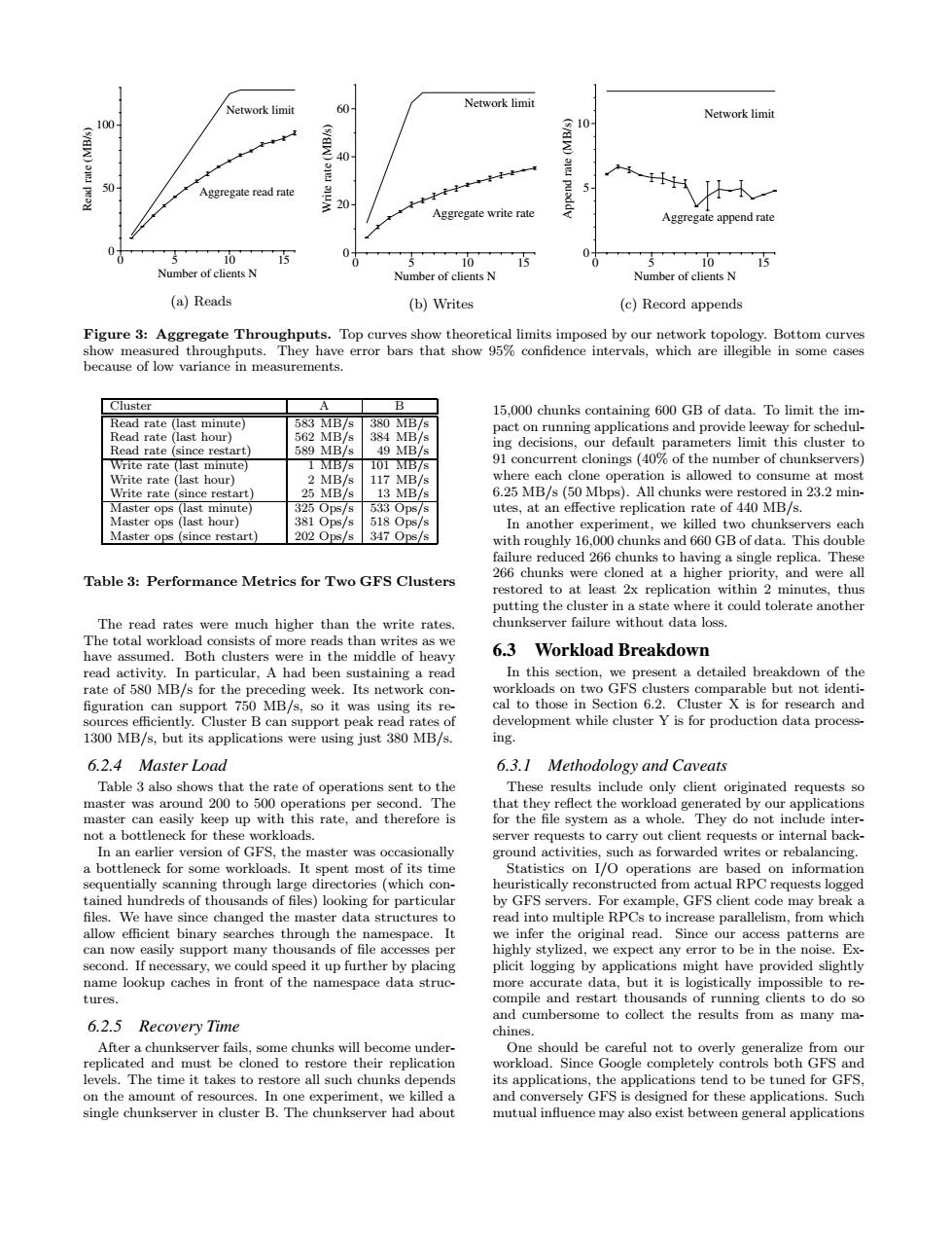
Network limit Network limit 60 Network limit 100 交10 40 50 Aggregate read rate 5 20 H人一 Aggregate write rate Aggregate append rate 10 15 0 5 0 10 15 5 10 15 Number of clients N Number of clients N Number of clients N (a)Reads (b)Writes (c)Record appends Figure 3:Aggregate Throughputs.Top curves show theoretical limits imposed by our network topology.Bottom curves show measured throughputs.They have error bars that show 95%confidence intervals,which are illegible in some cases because of low variance in measurements. Cluster A B 15,000 chunks containing 600 GB of data.To limit the im- Read rate (last minute) 583 MB/s 380 MB/s pact on running applications and provide leeway for schedul- Read rate(last hour） 562 MB/s 384 MB/s Read rate (since restart) 589 MB/s 49 MB/s ing decisions,our default parameters limit this cluster to Write rate (last minute) 1 MB/s 101B/s 91 concurrent clonings (40%of the number of chunkservers) Write rate (last hour) 2 MB/s 117 MB/s where each clone operation is allowed to consume at most Write rate (since restart) 25 MB/s 13 MB/s 6.25 MB/s (50 Mbps).All chunks were restored in 23.2 min- Master ops (last minute) 3250ps/s 5330ps/s utes,at an effective replication rate of 440 MB/s. Master ops (last hour) 381 Ops/s 518 Ops/s In another experiment,we killed two chunkservers each Master ops (since restart) 202 Ops/s 347 Ops/s with roughly 16.000 chunks and 660 GB of data.This double failure reduced 266 chunks to having a single replica.These Table 3:Performance Metrics for Two GFS Clusters 266 chunks were cloned at a higher priority,and were all restored to at least 2x replication within 2 minutes,thus putting the cluster in a state where it could tolerate another The read rates were much higher than the write rates. chunkserver failure without data loss. The total workload consists of more reads than writes as we have assumed.Both clusters were in the middle of heavy 6.3 Workload Breakdown read activity.In particular,A had been sustaining a read In this section,we present a detailed breakdown of the rate of 580 MB/s for the preceding week.Its network con- workloads on two GFS clusters comparable but not identi- figuration can support 750 MB/s,so it was using its re- cal to those in Section 6.2.Cluster X is for research and sources efficiently.Cluster B can support peak read rates of development while cluster Y is for production data process- 1300 MB/s,but its applications were using just 380 MB/s. ing. 6.2.4 Master Load 6.3.I Methodology and Caveats Table 3 also shows that the rate of operations sent to the These results include only client originated requests so master was around 200 to 500 operations per second.The that they reflect the workload generated by our applications master can easily keep up with this rate,and therefore is for the file system as a whole.They do not include inter- not a bottleneck for these workloads server requests to carry out client requests or internal back- In an earlier version of GFS,the master was occasionally ground activities,such as forwarded writes or rebalancing. a bottleneck for some workloads.It spent most of its time Statistics on I/O operations are based on information sequentially scanning through large directories (which con- heuristically reconstructed from actual RPC requests logged tained hundreds of thousands of files)looking for particular by GFS servers.For example,GFS client code may break a files.We have since changed the master data structures to read into multiple RPCs to increase parallelism,from which allow efficient binary searches through the namespace.It we infer the original read.Since our access patterns are can now easily support many thousands of file accesses per highly stylized,we expect any error to be in the noise.Ex- second.If necessary,we could speed it up further by placing plicit logging by applications might have provided slightly name lookup caches in front of the namespace data struc- more accurate data,but it is logistically impossible to re- tures. compile and restart thousands of running clients to do so and cumbersome to collect the results from as many ma- 6.2.5 Recovery Time chines. After a chunkserver fails,some chunks will become under- One should be careful not to overly generalize from our replicated and must be cloned to restore their replication workload.Since Google completely controls both GFS and levels.The time it takes to restore all such chunks depends its applications,the applications tend to be tuned for GFS, on the amount of resources.In one experiment,we killed a and conversely GFS is designed for these applications.Such single chunkserver in cluster B.The chunkserver had about mutual influence may also exist between general applications0 5 10 15 Number of clients N 0 50 100 Read rate (MB/s) Network limit Aggregate read rate (a) Reads 0 5 10 15 Number of clients N 0 20 40 60 Write rate (MB/s) Network limit Aggregate write rate (b) Writes 0 5 10 15 Number of clients N 0 5 10 Append rate (MB/s) Network limit Aggregate append rate (c) Record appends Figure 3: Aggregate Throughputs. Top curves show theoretical limits imposed by our networktopology. Bottom curves show measured throughputs. They have error bars that show 95% confidence intervals, which are illegible in some cases because of low variance in measurements. Cluster A B Read rate (last minute) 583 MB/s 380 MB/s Read rate (last hour) 562 MB/s 384 MB/s Read rate (since restart) 589 MB/s 49 MB/s Write rate (last minute) 1 MB/s 101 MB/s Write rate (last hour) 2 MB/s 117 MB/s Write rate (since restart) 25 MB/s 13 MB/s Master ops (last minute) 325 Ops/s 533 Ops/s Master ops (last hour) 381 Ops/s 518 Ops/s Master ops (since restart) 202 Ops/s 347 Ops/s Table 3: Performance Metrics for Two GFS Clusters The read rates were much higher than the write rates. The total workload consists of more reads than writes as we have assumed. Both clusters were in the middle of heavy read activity. In particular, A had been sustaining a read rate of 580 MB/s for the preceding week. Its network con- figuration can support 750 MB/s, so it was using its re￾sources efficiently. Cluster B can support peakread rates of 1300 MB/s, but its applications were using just 380 MB/s. 6.2.4 Master Load Table 3 also shows that the rate of operations sent to the master was around 200 to 500 operations per second. The master can easily keep up with this rate, and therefore is not a bottleneckfor these workloads. In an earlier version of GFS, the master was occasionally a bottleneckfor some workloads. It spent most of its time sequentially scanning through large directories (which con￾tained hundreds of thousands of files) looking for particular files. We have since changed the master data structures to allow efficient binary searches through the namespace. It can now easily support many thousands of file accesses per second. If necessary, we could speed it up further by placing name lookup caches in front of the namespace data struc￾tures. 6.2.5 Recovery Time After a chunkserver fails, some chunks will become under￾replicated and must be cloned to restore their replication levels. The time it takes to restore all such chunks depends on the amount of resources. In one experiment, we killed a single chunkserver in cluster B. The chunkserver had about 15,000 chunks containing 600 GB of data. To limit the im￾pact on running applications and provide leeway for schedul￾ing decisions, our default parameters limit this cluster to 91 concurrent clonings (40% of the number of chunkservers) where each clone operation is allowed to consume at most 6.25 MB/s (50 Mbps). All chunks were restored in 23.2 min￾utes, at an effective replication rate of 440 MB/s. In another experiment, we killed two chunkservers each with roughly 16,000 chunks and 660 GB of data. This double failure reduced 266 chunks to having a single replica. These 266 chunks were cloned at a higher priority, and were all restored to at least 2x replication within 2 minutes, thus putting the cluster in a state where it could tolerate another chunkserver failure without data loss. 6.3 Workload Breakdown In this section, we present a detailed breakdown of the workloads on two GFS clusters comparable but not identi￾cal to those in Section 6.2. Cluster X is for research and development while cluster Y is for production data process￾ing. 6.3.1 Methodology and Caveats These results include only client originated requests so that they reflect the workload generated by our applications for the file system as a whole. They do not include inter￾server requests to carry out client requests or internal back￾ground activities, such as forwarded writes or rebalancing. Statistics on I/O operations are based on information heuristically reconstructed from actual RPC requests logged by GFS servers. For example, GFS client code may breaka read into multiple RPCs to increase parallelism, from which we infer the original read. Since our access patterns are highly stylized, we expect any error to be in the noise. Ex￾plicit logging by applications might have provided slightly more accurate data, but it is logistically impossible to re￾compile and restart thousands of running clients to do so and cumbersome to collect the results from as many ma￾chines. One should be careful not to overly generalize from our workload. Since Google completely controls both GFS and its applications, the applications tend to be tuned for GFS, and conversely GFS is designed for these applications. Such mutual influence may also exist between general applications