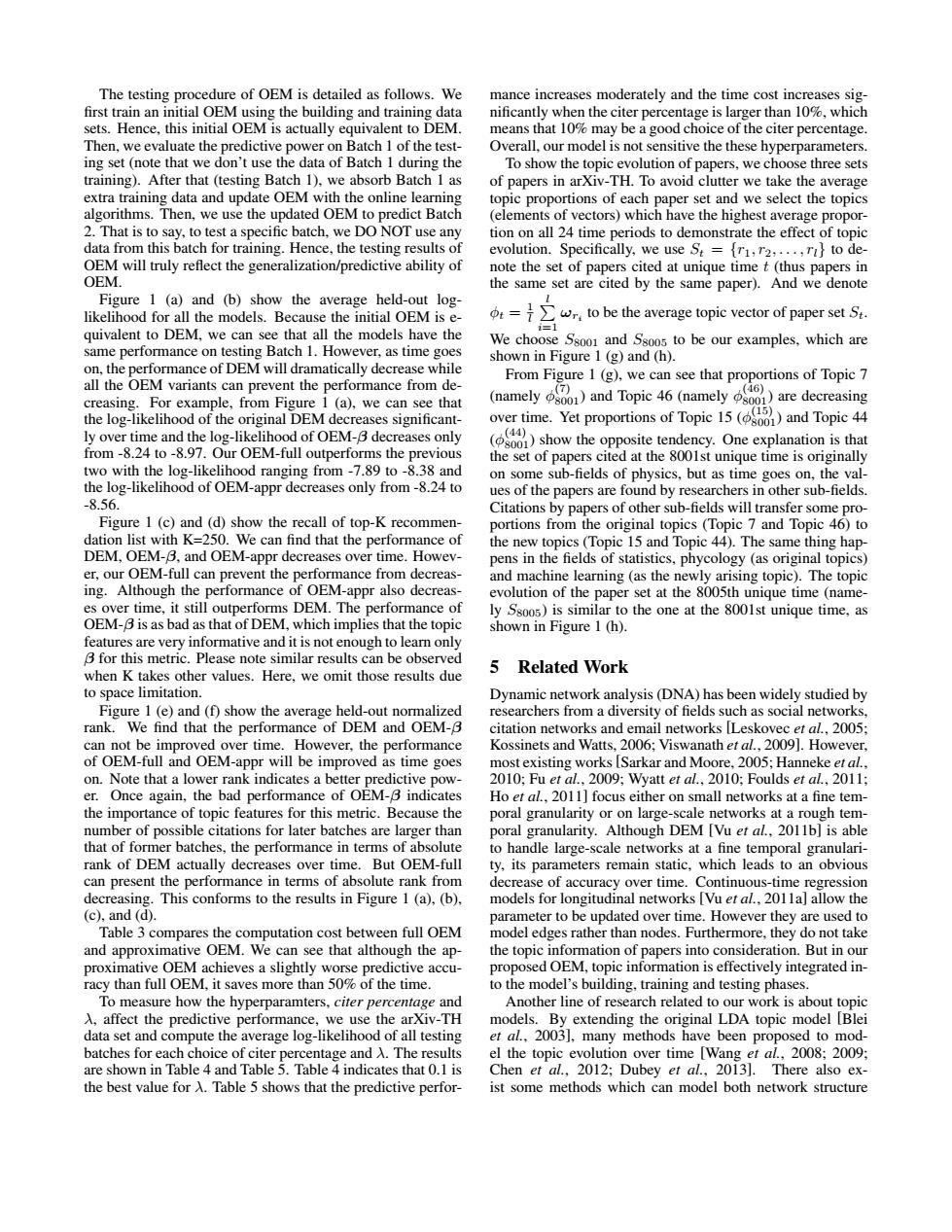
The testing procedure of OEM is detailed as follows.We mance increases moderately and the time cost increases sig- first train an initial OEM using the building and training data nificantly when the citer percentage is larger than 10%,which sets.Hence,this initial OEM is actually equivalent to DEM. means that 10%may be a good choice of the citer percentage. Then,we evaluate the predictive power on Batch 1 of the test- Overall,our model is not sensitive the these hyperparameters. ing set(note that we don't use the data of Batch I during the To show the topic evolution of papers,we choose three sets training).After that (testing Batch 1).we absorb Batch 1 as of papers in arXiv-TH.To avoid clutter we take the average extra training data and update OEM with the online learning topic proportions of each paper set and we select the topics algorithms.Then,we use the updated OEM to predict Batch (elements of vectors)which have the highest average propor- 2.That is to say,to test a specific batch,we DO NOT use any tion on all 24 time periods to demonstrate the effect of topic data from this batch for training.Hence,the testing results of evolution.Specifically,we use S.=[r1,r2,...,ri}to de- OEM will truly reflect the generalization/predictive ability of note the set of papers cited at unique time t(thus papers in OEM. the same set are cited by the same paper).And we denote Figure 1 (a)and (b)show the average held-out log- likelihood for all the models.Because the initial OEM is e- t=wr to be the average topic vector of paper set St. quivalent to DEM,we can see that all the models have the We choose Ssoor and Ssoos to be our examples,which are same performance on testing Batch 1.However,as time goes shown in Figure 1 (g)and (h). on,the performance of DEM will dramatically decrease while From Figure 1 (g),we can see that proportions of Topic 7 all the OEM variants can prevent the performance from de- creasing.For example,from Figure 1 (a),we can see that (namelyand Topic46 (namely are decreasing the log-likelihood of the original DEM decreases significant- over time.Yet proportions of Topic 15and Topic 44 ly over time and the log-likelihood of OEM-B decreases only )show the opposite tendency.One explanation is that from-8.24 to-8.97.Our OEM-full outperforms the previous the set of papers cited at the 8001st unique time is originally two with the log-likelihood ranging from-7.89 to -8.38 and on some sub-fields of physics,but as time goes on,the val- the log-likelihood of OEM-appr decreases only from-8.24 to ues of the papers are found by researchers in other sub-fields. -8.56. Citations by papers of other sub-fields will transfer some pro- Figure 1 (c)and (d)show the recall of top-K recommen- portions from the original topics (Topic 7 and Topic 46)to dation list with K=250.We can find that the performance of the new topics (Topic 15 and Topic 44).The same thing hap- DEM,OEM-B,and OEM-appr decreases over time.Howev- pens in the fields of statistics,phycology (as original topics) er,our OEM-full can prevent the performance from decreas- and machine learning (as the newly arising topic).The topic ing.Although the performance of OEM-appr also decreas- evolution of the paper set at the 8005th unique time(name- es over time,it still outperforms DEM.The performance of ly Ssoo5)is similar to the one at the 8001st unique time,as OEM-B is as bad as that of DEM,which implies that the topic shown in Figure 1 (h). features are very informative and it is not enough to learn only 3 for this metric.Please note similar results can be observed 5 Related Work when K takes other values.Here,we omit those results due to space limitation. Dynamic network analysis (DNA)has been widely studied by Figure 1 (e)and (f)show the average held-out normalized researchers from a diversity of fields such as social networks rank.We find that the performance of DEM and OEM-B citation networks and email networks Leskovec et al.,2005: can not be improved over time.However,the performance Kossinets and Watts.2006:Viswanath et al..2009.However. of OEM-full and OEM-appr will be improved as time goes most existing works [Sarkar and Moore,2005;Hanneke et al., on.Note that a lower rank indicates a better predictive pow- 2010;Fu et al.,2009;Wyatt et al.,2010;Foulds et al,2011; er.Once again,the bad performance of OEM-3 indicates Ho et al.,2011]focus either on small networks at a fine tem- the importance of topic features for this metric.Because the poral granularity or on large-scale networks at a rough tem- number of possible citations for later batches are larger than poral granularity.Although DEM [Vu et al.,2011b]is able that of former batches,the performance in terms of absolute to handle large-scale networks at a fine temporal granulari- rank of DEM actually decreases over time.But OEM-full ty,its parameters remain static,which leads to an obvious can present the performance in terms of absolute rank from decrease of accuracy over time.Continuous-time regression decreasing.This conforms to the results in Figure 1 (a),(b), models for longitudinal networks [Vu et al..201lal allow the (c),and (d). parameter to be updated over time.However they are used to Table 3 compares the computation cost between full OEM model edges rather than nodes.Furthermore,they do not take and approximative OEM.We can see that although the ap- the topic information of papers into consideration.But in our proximative OEM achieves a slightly worse predictive accu- proposed OEM,topic information is effectively integrated in- racy than full OEM,it saves more than 50%of the time. to the model's building,training and testing phases. To measure how the hyperparamters,citer percentage and Another line of research related to our work is about topic A,affect the predictive performance,we use the arXiv-TH models.By extending the original LDA topic model [Blei data set and compute the average log-likelihood of all testing et al.,2003],many methods have been proposed to mod- batches for each choice of citer percentage and A.The results el the topic evolution over time [Wang et al.,2008;2009; are shown in Table 4 and Table 5.Table 4 indicates that 0.1 is Chen et al.,2012;Dubey et al.,2013].There also ex- the best value for A.Table 5 shows that the predictive perfor- ist some methods which can model both network structureThe testing procedure of OEM is detailed as follows. We first train an initial OEM using the building and training data sets. Hence, this initial OEM is actually equivalent to DEM. Then, we evaluate the predictive power on Batch 1 of the test￾ing set (note that we don’t use the data of Batch 1 during the training). After that (testing Batch 1), we absorb Batch 1 as extra training data and update OEM with the online learning algorithms. Then, we use the updated OEM to predict Batch 2. That is to say, to test a specific batch, we DO NOT use any data from this batch for training. Hence, the testing results of OEM will truly reflect the generalization/predictive ability of OEM. Figure 1 (a) and (b) show the average held-out log￾likelihood for all the models. Because the initial OEM is e￾quivalent to DEM, we can see that all the models have the same performance on testing Batch 1. However, as time goes on, the performance of DEM will dramatically decrease while all the OEM variants can prevent the performance from de￾creasing. For example, from Figure 1 (a), we can see that the log-likelihood of the original DEM decreases significant￾ly over time and the log-likelihood of OEM-β decreases only from -8.24 to -8.97. Our OEM-full outperforms the previous two with the log-likelihood ranging from -7.89 to -8.38 and the log-likelihood of OEM-appr decreases only from -8.24 to -8.56. Figure 1 (c) and (d) show the recall of top-K recommen￾dation list with K=250. We can find that the performance of DEM, OEM-β, and OEM-appr decreases over time. Howev￾er, our OEM-full can prevent the performance from decreas￾ing. Although the performance of OEM-appr also decreas￾es over time, it still outperforms DEM. The performance of OEM-β is as bad as that of DEM, which implies that the topic features are very informative and it is not enough to learn only β for this metric. Please note similar results can be observed when K takes other values. Here, we omit those results due to space limitation. Figure 1 (e) and (f) show the average held-out normalized rank. We find that the performance of DEM and OEM-β can not be improved over time. However, the performance of OEM-full and OEM-appr will be improved as time goes on. Note that a lower rank indicates a better predictive pow￾er. Once again, the bad performance of OEM-β indicates the importance of topic features for this metric. Because the number of possible citations for later batches are larger than that of former batches, the performance in terms of absolute rank of DEM actually decreases over time. But OEM-full can present the performance in terms of absolute rank from decreasing. This conforms to the results in Figure 1 (a), (b), (c), and (d). Table 3 compares the computation cost between full OEM and approximative OEM. We can see that although the ap￾proximative OEM achieves a slightly worse predictive accu￾racy than full OEM, it saves more than 50% of the time. To measure how the hyperparamters, citer percentage and λ, affect the predictive performance, we use the arXiv-TH data set and compute the average log-likelihood of all testing batches for each choice of citer percentage and λ. The results are shown in Table 4 and Table 5. Table 4 indicates that 0.1 is the best value for λ. Table 5 shows that the predictive perfor￾mance increases moderately and the time cost increases sig￾nificantly when the citer percentage is larger than 10%, which means that 10% may be a good choice of the citer percentage. Overall, our model is not sensitive the these hyperparameters. To show the topic evolution of papers, we choose three sets of papers in arXiv-TH. To avoid clutter we take the average topic proportions of each paper set and we select the topics (elements of vectors) which have the highest average propor￾tion on all 24 time periods to demonstrate the effect of topic evolution. Specifically, we use St = {r1, r2, . . . , rl} to de￾note the set of papers cited at unique time t (thus papers in the same set are cited by the same paper). And we denote φt = 1 l P l i=1 ωri to be the average topic vector of paper set St. We choose S8001 and S8005 to be our examples, which are shown in Figure 1 (g) and (h). From Figure 1 (g), we can see that proportions of Topic 7 (namely φ (7) 8001) and Topic 46 (namely φ (46) 8001) are decreasing over time. Yet proportions of Topic 15 (φ (15) 8001) and Topic 44 (φ (44) 8001) show the opposite tendency. One explanation is that the set of papers cited at the 8001st unique time is originally on some sub-fields of physics, but as time goes on, the val￾ues of the papers are found by researchers in other sub-fields. Citations by papers of other sub-fields will transfer some pro￾portions from the original topics (Topic 7 and Topic 46) to the new topics (Topic 15 and Topic 44). The same thing hap￾pens in the fields of statistics, phycology (as original topics) and machine learning (as the newly arising topic). The topic evolution of the paper set at the 8005th unique time (name￾ly S8005) is similar to the one at the 8001st unique time, as shown in Figure 1 (h). 5 Related Work Dynamic network analysis (DNA) has been widely studied by researchers from a diversity of fields such as social networks, citation networks and email networks [Leskovec et al., 2005; Kossinets and Watts, 2006; Viswanath et al., 2009]. However, most existing works[Sarkar and Moore, 2005; Hanneke et al., 2010; Fu et al., 2009; Wyatt et al., 2010; Foulds et al., 2011; Ho et al., 2011] focus either on small networks at a fine tem￾poral granularity or on large-scale networks at a rough tem￾poral granularity. Although DEM [Vu et al., 2011b] is able to handle large-scale networks at a fine temporal granulari￾ty, its parameters remain static, which leads to an obvious decrease of accuracy over time. Continuous-time regression models for longitudinal networks [Vu et al., 2011a] allow the parameter to be updated over time. However they are used to model edges rather than nodes. Furthermore, they do not take the topic information of papers into consideration. But in our proposed OEM, topic information is effectively integrated in￾to the model’s building, training and testing phases. Another line of research related to our work is about topic models. By extending the original LDA topic model [Blei et al., 2003], many methods have been proposed to mod￾el the topic evolution over time [Wang et al., 2008; 2009; Chen et al., 2012; Dubey et al., 2013]. There also ex￾ist some methods which can model both network structure