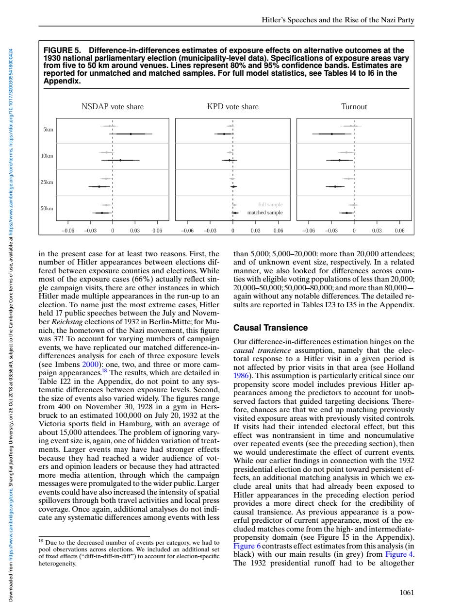
Hitler's Speeches and the Rise of the Nazi Party FIGURE 5.Difference-in-differences estimates of exposure effects on alternative outcomes at the 1930 national parliamentary election(municipality-level data).Specifications of exposure areas vary from five to 50 km around venues.Lines represent 80%and 95%confidence bands.Estimates are reported for unmatched and matched samples.For full model statistics,see Tables 14 to 16 in the Appendix. NSDAP vote share KPD vote share Turnout 5km 10km 25km full sample 50km matched sample -0.06 -0.03 0 0.03 0.06 -0.06 -0.03 0 0.03 0.06 -0.06-0.03 0 0.030.06 4r元 in the present case for at least two reasons.First,the than 5.000:5.000-20.000:more than 20.000 attendees: number of Hitler appearances between elections dif- and of unknown event size,respectively.In a related fered between exposure counties and elections.While manner,we also looked for differences across coun- most of the exposure cases (66%)actually reflect sin- ties with eligible voting populations of less than 20,000; gle campaign visits,there are other instances in which 20.000-50.000:50.000-80.000:and more than80.000- Hitler made multiple appearances in the run-up to an again without any notable differences.The detailed re- election.To name just the most extreme cases,Hitler sults are reported in Tables 123 to I35 in the Appendix. held 17 public speeches between the July and Novem- ber Reichstag elections of 1932 in Berlin-Mitte;for Mu- 是 nich,the hometown of the Nazi movement,this figure Causal Transience was 37!To account for varying numbers of campaign Our difference-in-differences estimation hinges on the events,we have replicated our matched difference-in- causal transience assumption,namely that the elec- differences analysis for each of three exposure levels toral response to a Hitler visit in a given period is 5795.801g (see Imbens 2000):one,two,and three or more cam- paign appearances.The results,which are detailed in not affected by prior visits in that area (see Holland Table 122 in the Appendix,do not point to any sys- 1986).This assumption is particularly critical since our tematic differences between exposure levels.Second. propensity score model includes previous Hitler ap- pearances among the predictors to account for unob- the size of events also varied widely.The figures range from 400 on November 30,1928 in a gym in Hers- served factors that guided targeting decisions.There- fore,chances are that we end up matching previously bruck to an estimated 100.000 on July 20,1932 at the Victoria sports field in Hamburg,with an average of visited exposure areas with previously visited controls. If visits had their intended electoral effect.but this about 15,000 attendees.The problem of ignoring vary- effect was nontransient in time and noncumulative ing event size is,again,one of hidden variation of treat- over repeated events(see the preceding section),then ments.Larger events may have had stronger effects we would underestimate the effect of current events. because they had reached a wider audience of vot- While our earlier findings in connection with the 1932 ers and opinion leaders or because they had attracted presidential election do not point toward persistent ef- more media attention,through which the campaign fects.an additional matching analysis in which we ex- messages were promulgated to the wider public.Larger clude areal units that had already been exposed to events could have also increased the intensity of spatial spillovers through both travel activities and local press Hitler appearances in the preceding election period provides a more direct check for the credibility of coverage.Once again,additional analyses do not indi- cate any systematic differences among events with less causal transience.As previous appearance is a pow- erful predictor of current appearance,most of the ex- cluded matches come from the high-and intermediate- 18 Due to the decreased number of events per category,we had to propensity domain(see Figure I5 in the Appendix). pool observations across elections.We included an additional set Figure 6 contrasts effect estimates from this analysis(in of fixed effects ("diff-in-diff-in-diff")to account for election-specific black)with our main results(in grey)from Figure 4. heterogeneity. The 1932 presidential runoff had to be altogether 1061Hitler’s Speeches and the Rise of the Nazi Party FIGURE 5. Difference-in-differences estimates of exposure effects on alternative outcomes at the 1930 national parliamentary election (municipality-level data). Specifications of exposure areas vary from five to 50 km around venues. Lines represent 80% and 95% confidence bands. Estimates are reported for unmatched and matched samples. For full model statistics, see Tables I4 to I6 in the Appendix. in the present case for at least two reasons. First, the number of Hitler appearances between elections dif￾fered between exposure counties and elections. While most of the exposure cases (66%) actually reflect sin￾gle campaign visits, there are other instances in which Hitler made multiple appearances in the run-up to an election. To name just the most extreme cases, Hitler held 17 public speeches between the July and Novem￾ber Reichstag elections of 1932 in Berlin-Mitte; for Mu￾nich, the hometown of the Nazi movement, this figure was 37! To account for varying numbers of campaign events, we have replicated our matched difference-in￾differences analysis for each of three exposure levels (see Imbens 2000): one, two, and three or more cam￾paign appearances.18 The results, which are detailed in Table I22 in the Appendix, do not point to any sys￾tematic differences between exposure levels. Second, the size of events also varied widely. The figures range from 400 on November 30, 1928 in a gym in Hers￾bruck to an estimated 100,000 on July 20, 1932 at the Victoria sports field in Hamburg, with an average of about 15,000 attendees. The problem of ignoring vary￾ing event size is, again, one of hidden variation of treat￾ments. Larger events may have had stronger effects because they had reached a wider audience of vot￾ers and opinion leaders or because they had attracted more media attention, through which the campaign messages were promulgated to the wider public.Larger events could have also increased the intensity of spatial spillovers through both travel activities and local press coverage. Once again, additional analyses do not indi￾cate any systematic differences among events with less 18 Due to the decreased number of events per category, we had to pool observations across elections. We included an additional set of fixed effects (“diff-in-diff-in-diff”) to account for election-specific heterogeneity. than 5,000; 5,000–20,000: more than 20,000 attendees; and of unknown event size, respectively. In a related manner, we also looked for differences across coun￾ties with eligible voting populations of less than 20,000; 20,000–50,000; 50,000–80,000; and more than 80,000— again without any notable differences. The detailed re￾sults are reported in Tables I23 to I35 in the Appendix. Causal Transience Our difference-in-differences estimation hinges on the causal transience assumption, namely that the elec￾toral response to a Hitler visit in a given period is not affected by prior visits in that area (see Holland 1986). This assumption is particularly critical since our propensity score model includes previous Hitler ap￾pearances among the predictors to account for unob￾served factors that guided targeting decisions. There￾fore, chances are that we end up matching previously visited exposure areas with previously visited controls. If visits had their intended electoral effect, but this effect was nontransient in time and noncumulative over repeated events (see the preceding section), then we would underestimate the effect of current events. While our earlier findings in connection with the 1932 presidential election do not point toward persistent ef￾fects, an additional matching analysis in which we ex￾clude areal units that had already been exposed to Hitler appearances in the preceding election period provides a more direct check for the credibility of causal transience. As previous appearance is a pow￾erful predictor of current appearance, most of the ex￾cluded matches come from the high- and intermediate￾propensity domain (see Figure I5 in the Appendix). Figure 6 contrasts effect estimates from this analysis (in black) with our main results (in grey) from Figure 4. The 1932 presidential runoff had to be altogether 1061 Downloaded from https://www.cambridge.org/core. Shanghai JiaoTong University, on 26 Oct 2018 at 03:56:49, subject to the Cambridge Core terms of use, available at https://www.cambridge.org/core/terms. https://doi.org/10.1017/S0003055418000424