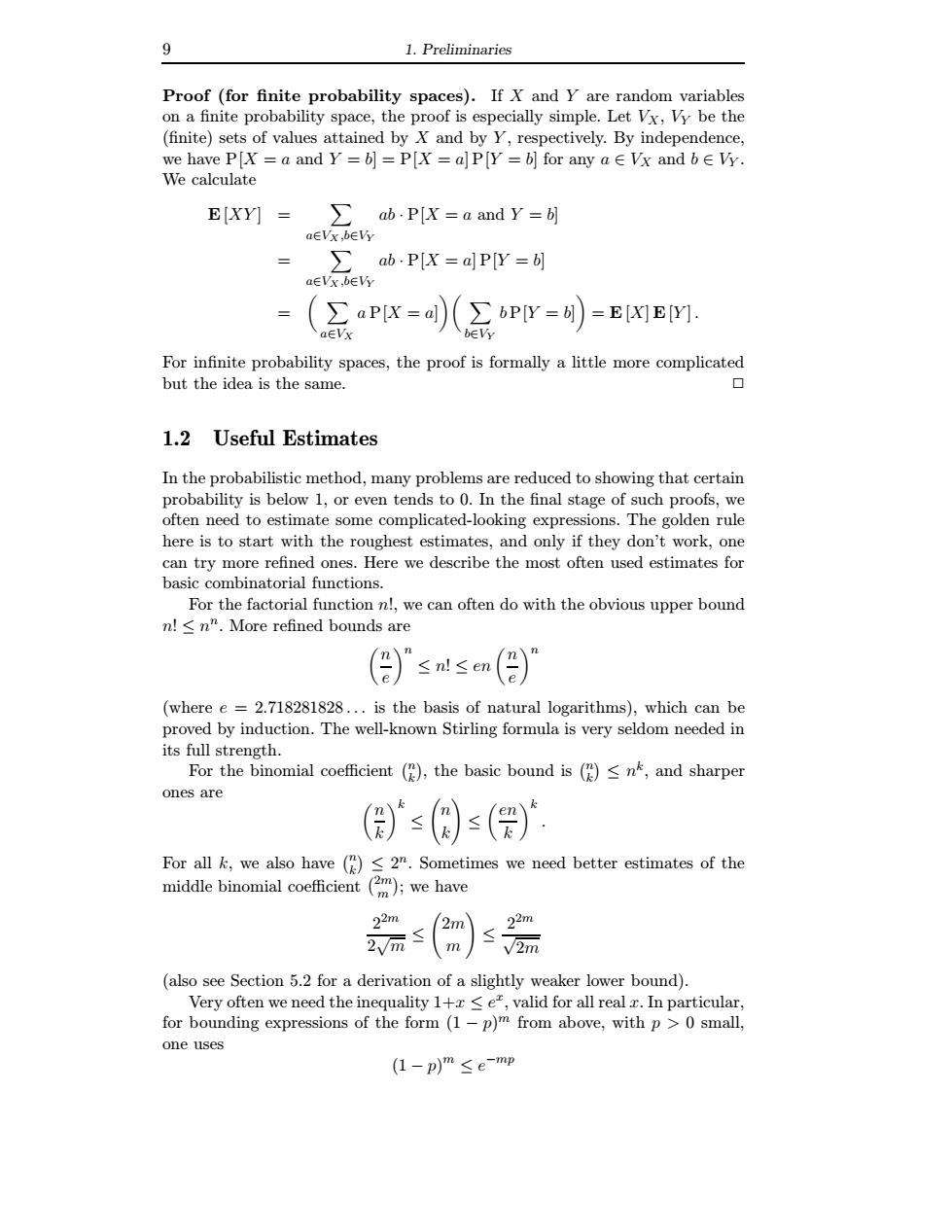
9 1.Preliminaries Proof(for finite probability spaces).If X and Y are random variables on a finite probability space,the proof is especially simple.Let Vx,Vy be the (finite)sets of values attained by X and by Y,respectively.By independence, we have P[X a and Y=]=P[X a]P[Y =b]for any a Vx and bVy. We calculate ∑ab.Px=a and y= = ab.P[X a]P[y =b = (∑aPX=al)(∑bPY=)=E[X]E [Y] aEVx but the idea is the same. 1.2 Useful Estimates th the probabilistic method,many problems are is belo 1,or even ten age of often nee e en rul here is to start ughest nd only i they don't can try ones. Here we describe the most often used estimates for basic co For the factorial function n!,we can often do with the obvious upper bound n!<n".More refined bounds are ()”s≤m()” =2.718281828 is the basis of natural ogarithms),which For the"o(月，the baic bound is(≤k,and sharper ones are ()≤（因s() For all k,we also have(2".Sometimes we need better estimates of the middle binomial coefficient ()we have 22m )需 (also see Section 5.2 for a derivation of a slightly weaker lower bound). Very often we nee d the inequality1+x≤e valid for all real In particula for bounding expressions of the form(1-p)from above,with p0small one uses (1-p)m≤e-mp 9 1. Preliminaries Proof (for finite probability spaces). If X and Y are random variables on a finite probability space, the proof is especially simple. Let VX, VY be the (finite) sets of values attained by X and by Y , respectively. By independence, we have P[X = a and Y = b] = P[X = a] P[Y = b] for any a ∈ VX and b ∈ VY . We calculate E [XY ] = X a∈VX ,b∈VY ab · P[X = a and Y = b] = X a∈VX ,b∈VY ab · P[X = a] P[Y = b] =  X a∈VX a P[X = a]  X b∈VY b P[Y = b]  = E [X] E [Y ] . For infinite probability spaces, the proof is formally a little more complicated but the idea is the same. ✷ 1.2 Useful Estimates In the probabilistic method, many problems are reduced to showing that certain probability is below 1, or even tends to 0. In the final stage of such proofs, we often need to estimate some complicated-looking expressions. The golden rule here is to start with the roughest estimates, and only if they don’t work, one can try more refined ones. Here we describe the most often used estimates for basic combinatorial functions. For the factorial function n!, we can often do with the obvious upper bound n! ≤ n n . More refined bounds are  n e n ≤ n! ≤ en  n e n (where e = 2.718281828 . . . is the basis of natural logarithms), which can be proved by induction. The well-known Stirling formula is very seldom needed in its full strength. For the binomial coefficient ￾n k
, the basic bound is ￾n k
≤ n k , and sharper ones are  n k k ≤ n k ! ≤  en k k . For all k, we also have ￾n k
≤ 2 n . Sometimes we need better estimates of the middle binomial coefficient ￾ 2m m
; we have 2 2m 2 √ m ≤ 2m m ! ≤ 2 2m √ 2m (also see Section 5.2 for a derivation of a slightly weaker lower bound). Very often we need the inequality 1+x ≤ e x , valid for all real x. In particular, for bounding expressions of the form (1 − p) m from above, with p > 0 small, one uses (1 − p) m ≤ e −mp