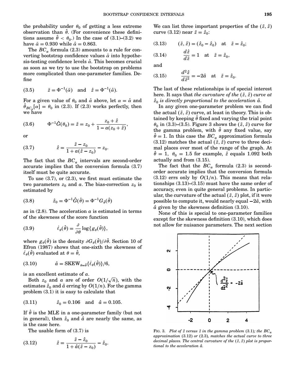
BOOTSTRAP CONFIDENCE INTERVALS 195 the probability under 0o of getting a less extreme We can list three important properties of the(2,2) observation than 0.(For convenience these defini- curve (3.12)near=20: tions assume <00.)In the case of(3.1)-(3.2)we have a=0.930 while a=0.863. (3.13) (2,)=(2o-0)at乏=o: The BCa formula(2.3)amounts to a rule for con- verting bootstrap confidence values into hypothe- (3.14) dE=1at2=0, sis-testing confidence levels a.This becomes crucial as soon as we try to use the bootstrap on problems and more complicated than one-parameter families.De- d22 (3.15) fine d2=-2d at. (3.5) z=Φ-(a)ande=Φ-1(a) The last of these relationships is of special interest here.It says that the curvature of the (z,2)curve at For a given value of 0o and a above,let a=a and 20 is directly proportional to the acceleration a. eBC [a]0o in (2.3).If (2.3)works perfectly,then In any given one-parameter problem we can find we have the actual(2,2)curve,at least in theory.This is ob- tained by keeping 6 fixed and varying the trial point (3.6) 20十2 Φ-1G(00)=2=20+1-a(20+) 0o in (3.3)-(3.5).Figure 3 shows the (2,2)curve for the gamma problem,with 6 any fixed value,say or =1.In this case the BC approximation formula (3.7) 2-20 (3.12)matches the actual(,2)curve to three deci- 龙=1+a(2-z0) -20 mal places over most of the range of the graph.At 0=1,00 1.5 for example,2 equals 1.092 both The fact that the BC intervals are second-order actually and from(3.15). accurate implies that the conversion formula(3.7) The fact that the BCa formula(2.3)is second- itself must be quite accurate. order accurate implies that the conversion formula To use (3.7),or(2.3),we first must estimate the (3.12)errs only by O(1/n).This means that rela- two parameters zo and a.The bias-correction zo is tionships (3.13)-(3.15)must have the same order of estimated by accuracy,even in quite general problems.In partic- ular,the curvature of the actual(,)plot,if it were (3.8) 0=Φ-1G(0)=-1G(0 possible to compute it,would nearly equal-2a,with a given by the skewness definition(3.10). as in(2.8).The acceleration a is estimated in terms None of this is special to one-parameter families of the skewness of the score function except for the skewness definition(3.10),which does (3.9) o=品1g{g.(o, not allow for nuisance parameters.The next section where ge(0)is the density Ge(0)/00.Section 10 of Efron (1987)shows that one-sixth the skewness of (0)evaluated at 0=6, (3.10) a =SKEW0-oflo(0)}/6, is an excellent estimate of a. Both zo and a are of order O(1/n),with the estimates 2o and a erring by O(1/n).For the gamma problem(3.1)it is easy to calculate that (3.11) 20=0.106anda=0.105. If 6 is the MLE in a one-parameter family (but not in general),then 2o and d are nearly the same,as 2 0 2 is the case here. The usable form of(3.7)is FIG.3.Plot of versus in the gamma problem (3.1);the BC approximation (3.12)or(2.3),matches the actual curve to three (3.12) 2-20 2= decimal places.The central curvature of the(2,2)plot is propor 1+(2-20) -0 tional to the acceleration a.BOOTSTRAP CONFIDENCE INTERVALS 195 the probability under θ0 of getting a less extreme observation than θˆ. (For convenience these defini￾tions assume θˆ < θ0 .) In the case of (3.1)–(3.2) we have α˜ = 0:930 while αˆ = 0:863. The BCa formula (2.3) amounts to a rule for con￾verting bootstrap confidence values α˜ into hypothe￾sis-testing confidence levels αˆ. This becomes crucial as soon as we try to use the bootstrap on problems more complicated than one-parameter families. De- fine 3:5‘ z˜ = 8 −1 α˜‘ and zˆ = 8 −1 αˆ‘: For a given value of θ0 and αˆ above, let α = αˆ and θˆBCa ’α = θ0 in (2.3). If (2.3) works perfectly, then we have 3:6‘ 8 −1Gˆ θ0 ‘ = z˜ = z0 + z0 + zˆ 1 − az0 + zˆ‘ ; or 3:7‘ zˆ = z˜ − z0 1 + azˆ − z0 ‘ − z0 : The fact that the BCa intervals are second-order accurate implies that the conversion formula (3.7) itself must be quite accurate. To use (3.7), or (2.3), we first must estimate the two parameters z0 and a. The bias-correction z0 is estimated by 3:8‘ zˆ0 = 8 −1Gˆ θˆ‘ = 8 −1Gθˆθˆ‘ as in (2.8). The acceleration a is estimated in terms of the skewness of the score function 3:9‘ `˙ θ θˆ‘ = ∂ ∂θ loggθ θˆ‘•; where gθ θˆ‘ is the density ∂Gθ θˆ‘/∂θˆ. Section 10 of Efron (1987) shows that one-sixth the skewness of `˙ θ θˆ‘ evaluated at θ = θˆ, 3:10‘ aˆ = SKEWθ=θˆ`˙ θ θˆ‘•/6; is an excellent estimate of a. Both z0 and a are of order O1/ √ n‘, with the estimates zˆ0 and aˆ erring by O1/n‘. For the gamma problem (3.1) it is easy to calculate that 3:11‘ zˆ0 = 0:106 and aˆ = 0:105: If θˆ is the MLE in a one-parameter family (but not in general), then zˆ0 and aˆ are nearly the same, as is the case here. The usable form of (3.7) is 3:12‘ zˆ = z˜ − zˆ0 1 + aˆz˜ − z0 ‘ − zˆ0 : We can list three important properties of the z˜; zˆ‘ curve (3.12) near z˜ = zˆ0 : z˜; zˆ‘ = zˆ0 − zˆ0 ‘ at z˜ = zˆ0 (3.13) y dzˆ dz˜ = 1 at z˜ = zˆ0 (3.14) ; and d 2zˆ dz˜ 2 = −2aˆ at z˜ = zˆ0 (3.15) : The last of these relationships is of special interest here. It says that the curvature of the z˜; zˆ‘ curve at zˆ0 is directly proportional to the acceleration aˆ. In any given one-parameter problem we can find the actual z˜; zˆ‘ curve, at least in theory. This is ob￾tained by keeping θˆ fixed and varying the trial point θ0 in (3.3)–(3.5). Figure 3 shows the z˜; zˆ‘ curve for the gamma problem, with θˆ any fixed value, say θˆ = 1. In this case the BCa approximation formula (3.12) matches the actual z˜; zˆ‘ curve to three deci￾mal places over most of the range of the graph. At θˆ = 1; θ0 = 1:5 for example, zˆ equals 1.092 both actually and from (3.15). The fact that the BCa formula (2.3) is second￾order accurate implies that the conversion formula (3.12) errs only by O1/n‘. This means that rela￾tionships (3.13)–(3.15) must have the same order of accuracy, even in quite general problems. In partic￾ular, the curvature of the actual z˜; zˆ‘ plot, if it were possible to compute it, would nearly equal −2aˆ, with aˆ given by the skewness definition (3.10). None of this is special to one-parameter families except for the skewness definition (3.10), which does not allow for nuisance parameters. The next section Fig. 3. Plot of zˆ versus z˜ in the gamma problem 3:1‘; the BCa approximation 3:12‘ or 2:3‘, matches the actual curve to three decimal places. The central curvature of the z˜; zˆ‘ plot is propor￾tional to the acceleration aˆ.