If we use the distribution functions with k=1 to fit the data, (ii)Consider a generalised normal family the p-value for the test is 0.03-much more significant than that 2-1-1/k a)=r+加{- under the assumption of normal distribution. which has the mean u.When k=2,it is N(u,2). (iii)The empirical likelihood ratio test statistic 2logT 3.56, which rejects Ho with the p-value 0.04. To find the profile likelihood of u,the 'MLE'for a is The 95%confidence interval is ==克2X-4 15 2n1 {μ∑1og()>-1.92-15Iog(15)月=0.17,4.27]. =1 Hence ()=(n,a)=-nlogr(1+-n(1+)l0g2-nloga- The DE density is of the formel/.With fixed,the MLE for o is nX;-.Hence the parametric log (profile) Fig.(b)shows the MLE=(k)varies with respect to k.In fact likelihood is (k)increases as k decreases. -nlog∑IX:-4 3.Empirical likelihood for random vectors Let X1,...:Xn be i.i.d.random vectors from distribution F. Similar to the univariate case,we assume pi=F(X),i=1,…,n, where pi0 and ipi=1.The empirical likelihood is L(pm1,…,pPm)=Πn 2=1 Parametric log-likelihood (solid curve)based on the DE distribu- Without any further constraints,the MELEs are tion,and the empirical log-likelihood(dashed curve).(Both curves i=1/m,i=1,…,n. were shifted vertically by their own maximum values.(ii) Consider a generalised normal family fk(x|µ, σ) = 2 −1−1/k Γ(1 + 1/k)σ exp  − 1 2     x − µ σ     k , which has the mean µ. When k = 2, it is N(µ, σ2). To find the profile likelihood of µ, the ‘MLE’ for σ is σb k ≡ σb(µ) k = k 2n Xn i=1 |Xi − µ| k . Hence lk(µ) = lk(µ, σb) = −n log Γ(1 + 1 k ) − n(1 + 1 k ) log 2 − n log σb − n k . Fig.(b) shows the MLE µb = µb(k) varies with respect to k. In fact µb(k) increases as k decreases. If we use the distribution functions with k = 1 to fit the data, the p-value for the test is 0.03 – much more significant than that under the assumption of normal distribution. (iii) The empirical likelihood ratio test statistic 2 log T = 3.56, which rejects H0 with the p-value 0.04. 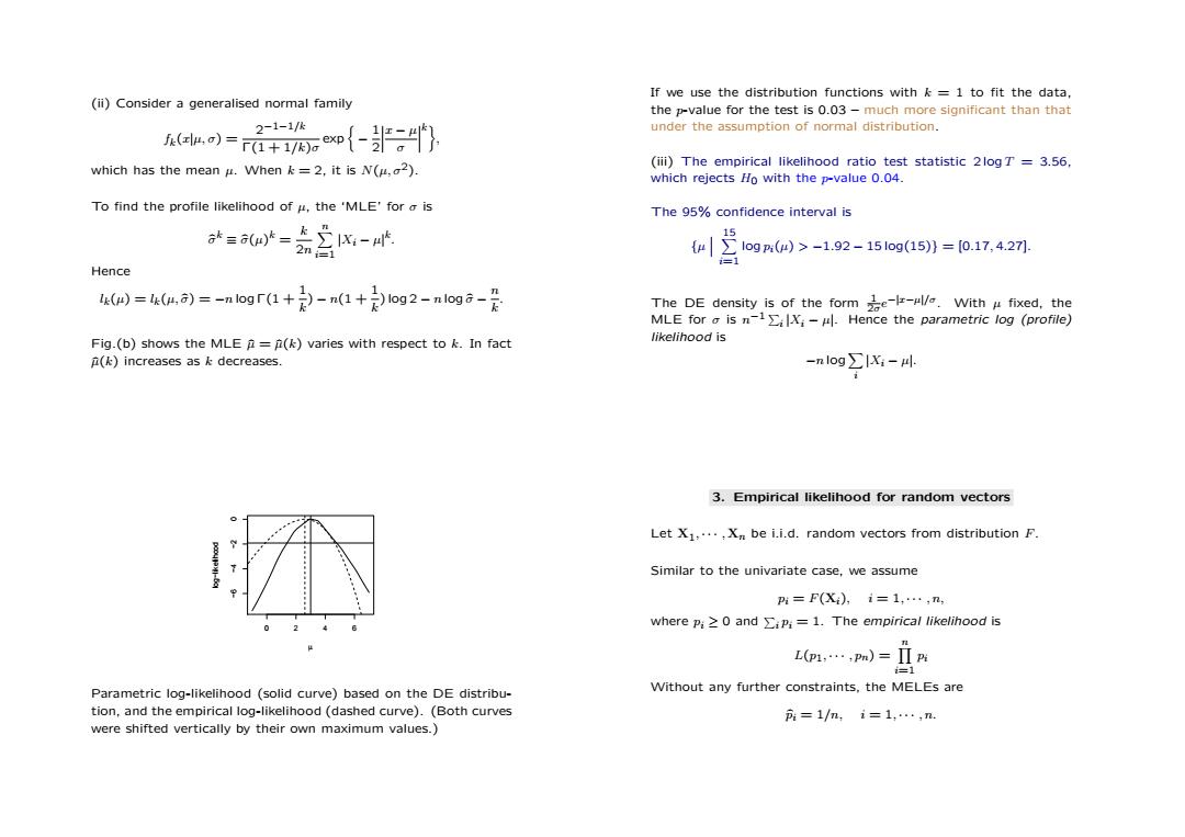The 95% confidence interval is {µ    X 15 i=1 log pi(µ) > −1.92 − 15 log(15)} = [0.17, 4.27]. The DE density is of the form 1 2σ e −|x−µ|/σ. With µ fixed, the MLE for σ is n −1 P i |Xi − µ|. Hence the parametric log (profile) likelihood is −n logX i |Xi − µ|. 0 2 4 6 −6 −4 −2 0 µ log−likelihood Parametric log-likelihood (solid curve) based on the DE distribu￾tion, and the empirical log-likelihood (dashed curve). (Both curves were shifted vertically by their own maximum values.) 3. Empirical likelihood for random vectors Let X1, · · · , Xn be i.i.d. random vectors from distribution F. Similar to the univariate case, we assume pi = F(Xi), i = 1, · · · , n, where pi ≥ 0 and P i pi = 1. The empirical likelihood is L(p1, · · · , pn) = Yn i=1 pi Without any further constraints, the MELEs are pbi = 1/n, i = 1, · · · , n