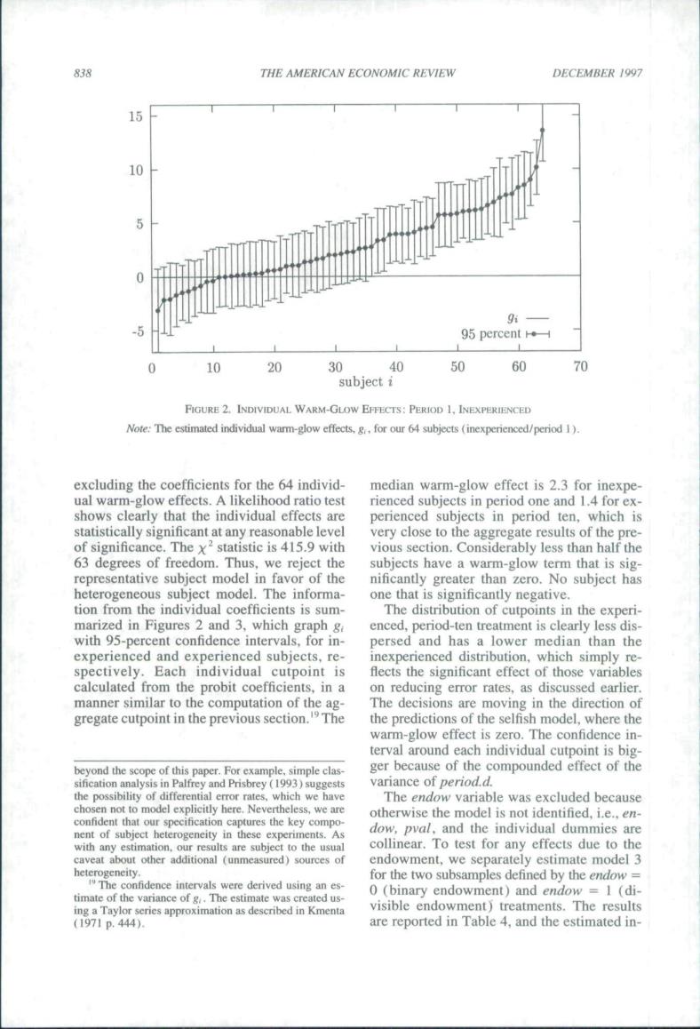
THE AMERICAN ECONOMIC REVIEW DECEMBER 1997 15 10 0 10 20 30 0 50 60 70 subject i FIGURE 2.INDIVIDUAL WARM-GLOW EFFECTS:PERIOD 1.INEXPERIENCED Note:The estimated individual warm-glow effects.for our 64 subjects(inexperienced/period 1) median warm-glow effect is 2.3 for shows clearly that the individual effects are perienced subiects in period ten.which is statisificaneg tistie is415.9 with very close to the aggregate results of the pre The x'sta vious section.Considerably less than half egree ive suhieet mo heterogeneous subject model.The informa- one that is significantly negative. tion from the e individual coefh ents is sum The distribution of cutpoints in the experi- enced. ten tre tment is c arly which sim spectively. Each individual cutpoint is flects the significant effect of those variables calculated f probit co in a on reducing error rates,as di cussed earlier warm-glow effect is zero.The confidence in. terval around each individual cutpoint is big- nd the s imnle clas ger because of the compounded effect of the nd Pri e was excluded hecaus ures the key otherwise the model is not identified.i.e..en and the individual dummies ar o the collinear. To test for any ettects due to timate of the ing an c 0(binary endowment)and endow =1(di- n as described in Km visible end 4.and the estimated in838 THE AMERICAN ECONOMIC REVIEW DECEMBER 1997 15 - 10 - 5 ~ -p^T￾T T .•••'•' n TTTTTTTT ..-^-^^^'^ 0 ----,----n^-- j-j^ - . -5 '-Li 1 J --'llpp^^ 95 percent t-«-H 10 20 30 40 subject i 50 60 70 FIGURE 2, iNDtviDUAL WARM-GLOW EFFECTS: PERIOD 1, INEXPERIENCED Nole: The estimated individual warm-glow effects, g,, for our 64 subjects (inexperienced/period 1). excluding the coefficients for the 64 individ￾ual warm-glow effects. A likelihood ratio test shows clearly that the individual effects are statistically significant at any reasonable level of significance. The x^ statistic is 415.9 with 63 degrees of freedom. Thus, we reject the representative subject model in favor of the heterogeneous subject model. The informa￾tion from the individual coefficients is sum￾marized in Figures 2 and 3, which graph g, with 95-percent confidence intervals, for in￾experienced and experienced subjects, re￾spectively. Each individual cutpoint is calculated from the probit coefficients, in a manner similar to the computation of the ag￾gregate cutpoint in the previous section.'" The beyond the scope of this paper. For example, simple clas￾sification analysis in Palfrey and Prisbrey (1993) suggests the possibility of differential error rates, which we have chosen not to model explicitly here. Nevertheless, we are confident that our specification captures the key compo￾nent of subject heterogeneity in these experiments. As with any estimation, our results are subject to the usual caveat about other additional (unmeasured) sources of heterogeneity. '"The confidence intervals were derived using an es￾timate of the variance of g,. The estimate was created us￾ing a Taylor series approximation as described in Kmenta (1971 p. 444). median warm-glow effect is 2,3 for inexpe￾rienced subjects in period one and 1.4 for ex￾perienced subjects in period ten, which is very close to the aggregate results of the pre￾vious section. Considerably less than half the subjects have a warm-glow term that is sig￾nificantly greater than zero. No subject has one that is significantly negative. The distribution of cutpoints in the experi￾enced, period-ten treatment is clearly less dis￾persed and has a lower median than the inexperienced distribution, which simply re￾flects the significant effect of those variables on reducing error rates, as discussed earlier. The decisions are moving in the direction of the predictions of the selfish model, where the warm-glow effect is zero. The confidence in￾terval around each individual cutpoint is big￾ger because of the compounded effect of the variance of period.d. The endow variable was excluded because otherwise the model is not identified, i.e,, en￾dow, pval, and the individual dummies are collinear. To test for any effects due to the endowment, we separately estimate model 3 for the two subsamples defined by the endow = 0 (binary endowment) and endow = I (di￾visible endowment) treatments. The results are reported in Table 4, and the estimated in-