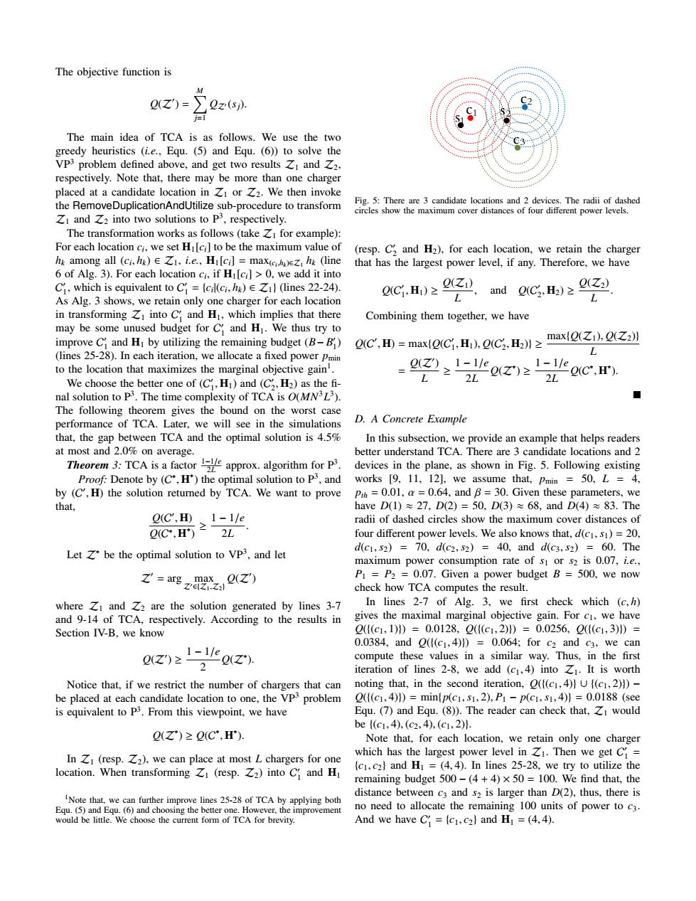
The objective function is M Q(Z')= Qz (sj). The main idea of TCA is as follows.We use the two C3 greedy heuristics (i.e.,Equ.(5)and Equ.(6))to solve the VP3 problem defined above,and get two results Z1 and Z2. respectively.Note that,there may be more than one charger placed at a candidate location in Zi or Z2.We then invoke the RemoveDuplicationAndUtilize sub-procedure to transform Fig.5:There are 3 candidate locations and 2 devices.The radii of dashed circles show the maximum cover distances of four different power levels. ZI and Z2 into two solutions to p3,respectively. The transformation works as follows (take ZI for example): For each location ci,we set Hi[ci]to be the maximum value of (resp.C and H2),for each location,we retain the charger hg among all (ci,hg)EZ1,i.e.,Hi[ci]max(ehez hg (line that has the largest power level,if any.Therefore,we have 6 of Alg.3).For each location ci,if Hi[ci]>0,we add it into C.which is equivalent to C=(cil(ci,h)EZi)(lines 22-24). As Alg.3 shows,we retain only one charger for each location Qc,≥，dQc≥2 L in transforming Zi into C and H,which implies that there Combining them together.we have may be some unused budget for C and H1.We thus try to improve C and HI by utilizing the remaining budget(B-B) 2C,田=max0C,H.Q(C2,H≥max0z(z2》 (lines 25-28).In each iteration,we allocate a fixed power Pmin L to the location that maximizes the marginal objective gain. 2≥lezz'acr L We choose the better one of (C.H1)and (C2.H2)as the fi- nal solution to P3.The time complexity of TCA is O(MN3L3). The following theorem gives the bound on the worst case performance of TCA.Later,we will see in the simulations D.A Concrete Example that,the gap between TCA and the optimal solution is 4.5% In this subsection,we provide an example that helps readers at most and 2.0%on average. better understand TCA.There are 3 candidate locations and 2 Theorem 3:TCA is a factor approx.algorithm for P3 devices in the plane,as shown in Fig.5.Following existing Proof:Denote by (C',H')the optimal solution to p3,and works [9,11,12],we assume that,pmin 50,L 4. by (C',H)the solution returned by TCA.We want to prove Ph=0.01,a=0.64,and B=30.Given these parameters,we that, have D1)≈27，D2)=50,D(3)≈68，andD(4)≈83.The Q(C,田、1-1/e radii of dashed circles show the maximum cover distances of QC,Hr≥ 2L four different power levels.We also knows that,d(c1,s1)=20, Let Z'be the optimal solution to VP3,and let dc1,s2)=70,dc2,s2)=40,andd(c3,s2)=60.The maximum power consumption rate of si or s2 is 0.07,i.e., arg() P1 =P2 =0.07.Given a power budget B =500,we now check how TCA computes the result. where Zi and Z2 are the solution generated by lines 3-7 In lines 2-7 of Alg.3,we first check which (c,h) and 9-14 of TCA,respectively.According to the results in gives the maximal marginal objective gain.For cI,we have Section IV-B,we know Q{(c1,1)）=0.0128.Q(c1,2)》=0.0256,Q({(c1,3)》）= 0.0384,and ([(c1,4)))=0.064;for c2 and c3,we can ez≥1-，1yez compute these values in a similar way.Thus,in the first 2 iteration of lines 2-8,we add (c1,4)into Z1.It is worth Notice that,if we restrict the number of chargers that can noting that,in the second iteration,(((c1,4)U((c1,2)))- be placed at each candidate location to one,the Vp3 problem Q(c1,4)D=mintp(c1,s1,2),P-pc1,s1,4)}=0.0188(see is equivalent to P3.From this viewpoint,we have Equ.(7)and Equ.(8)).The reader can check that,Zi would be{(c1,4),(c2,4),(c1,2)h. (Z)>(C'.H). Note that,for each location,we retain only one charger In Z (resp.Z2),we can place at most L chargers for one which has the largest power level in Z1.Then we get C= location.When transforming Z (resp.Z2)into C and H (c1,c2}and H =(4,4).In lines 25-28,we try to utilize the remaining budget 500-(4+4)x 50 =100.We find that,the INote that,we can further improve lines 25-28 of TCA by applying both distance between c3 and s2 is larger than D(2),thus,there is Equ.(5)and Equ.(6)and choosing the better one.However,the improvement no need to allocate the remaining 100 units of power to c3. would be little.We choose the current form of TCA for brevity. And we have C=(c1,c2}and H1=(4,4).The objective function is Q(Z′ ) = ∑ M j=1 QZ′ (sj). The main idea of TCA is as follows. We use the two greedy heuristics (i.e., Equ. (5) and Equ. (6)) to solve the VP3 problem defined above, and get two results Z1 and Z2, respectively. Note that, there may be more than one charger placed at a candidate location in Z1 or Z2. We then invoke the RemoveDuplicationAndUtilize sub-procedure to transform Z1 and Z2 into two solutions to P3 , respectively. The transformation works as follows (take Z1 for example): For each location ci , we set H1[ci] to be the maximum value of hk among all (ci , hk) ∈ Z1, i.e., H1[ci] = max(ci ,hk )∈Z1 hk (line 6 of Alg. 3). For each location ci , if H1[ci] > 0, we add it into C ′ 1 , which is equivalent to C ′ 1 = {ci |(ci , hk) ∈ Z1} (lines 22-24). As Alg. 3 shows, we retain only one charger for each location in transforming Z1 into C ′ 1 and H1, which implies that there may be some unused budget for C ′ 1 and H1. We thus try to improve C ′ 1 and H1 by utilizing the remaining budget (B− B ′ 1 ) (lines 25-28). In each iteration, we allocate a fixed power pmin to the location that maximizes the marginal objective gain1 . We choose the better one of (C ′ 1 , H1) and (C ′ 2 , H2) as the fi- nal solution to P3 . The time complexity of TCA is O(MN3L 3 ). The following theorem gives the bound on the worst case performance of TCA. Later, we will see in the simulations that, the gap between TCA and the optimal solution is 4.5% at most and 2.0% on average. Theorem 3: TCA is a factor 1−1/e 2L approx. algorithm for P3 . Proof: Denote by (C ∗ , H ∗ ) the optimal solution to P3 , and by (C ′ , H) the solution returned by TCA. We want to prove that, Q(C ′ , H) Q(C∗ , H ∗ ) ≥ 1 − 1/e 2L . Let Z∗ be the optimal solution to VP3 , and let Z′ = arg max Z′∈{Z1,Z2} Q(Z′ ) where Z1 and Z2 are the solution generated by lines 3-7 and 9-14 of TCA, respectively. According to the results in Section IV-B, we know Q(Z′ ) ≥ 1 − 1/e 2 Q(Z∗ ). Notice that, if we restrict the number of chargers that can be placed at each candidate location to one, the VP3 problem is equivalent to P3 . From this viewpoint, we have Q(Z∗ ) ≥ Q(C ∗ , H ∗ ). In Z1 (resp. Z2), we can place at most L chargers for one location. When transforming Z1 (resp. Z2) into C ′ 1 and H1 1Note that, we can further improve lines 25-28 of TCA by applying both Equ. (5) and Equ. (6) and choosing the better one. However, the improvement would be little. We choose the current form of TCA for brevity. c1 s2 s1 c2 c3 Fig. 5: There are 3 candidate locations and 2 devices. The radii of dashed circles show the maximum cover distances of four different power levels. (resp. C ′ 2 and H2), for each location, we retain the charger that has the largest power level, if any. Therefore, we have Q(C ′ 1 , H1) ≥ Q(Z1) L , and Q(C ′ 2 , H2) ≥ Q(Z2) L . Combining them together, we have Q(C ′ , H) = max{Q(C ′ 1 , H1), Q(C ′ 2 , H2)} ≥ max{Q(Z1), Q(Z2)} L = Q(Z′ ) L ≥ 1 − 1/e 2L Q(Z∗ ) ≥ 1 − 1/e 2L Q(C ∗ , H ∗ ). D. A Concrete Example In this subsection, we provide an example that helps readers better understand TCA. There are 3 candidate locations and 2 devices in the plane, as shown in Fig. 5. Following existing works [9, 11, 12], we assume that, pmin = 50, L = 4, pth = 0.01, α = 0.64, and β = 30. Given these parameters, we have D(1) ≈ 27, D(2) = 50, D(3) ≈ 68, and D(4) ≈ 83. The radii of dashed circles show the maximum cover distances of four different power levels. We also knows that, d(c1, s1) = 20, d(c1, s2) = 70, d(c2, s2) = 40, and d(c3, s2) = 60. The maximum power consumption rate of s1 or s2 is 0.07, i.e., P1 = P2 = 0.07. Given a power budget B = 500, we now check how TCA computes the result. In lines 2-7 of Alg. 3, we first check which (c, h) gives the maximal marginal objective gain. For c1, we have Q({(c1, 1)}) = 0.0128, Q({(c1, 2)}) = 0.0256, Q({(c1, 3)}) = 0.0384, and Q({(c1, 4)}) = 0.064; for c2 and c3, we can compute these values in a similar way. Thus, in the first iteration of lines 2-8, we add (c1, 4) into Z1. It is worth noting that, in the second iteration, Q({(c1, 4)} ∪ {(c1, 2)}) − Q({(c1, 4)}) = min{p(c1, s1, 2), P1 − p(c1, s1, 4)} = 0.0188 (see Equ. (7) and Equ. (8)). The reader can check that, Z1 would be {(c1, 4), (c2, 4), (c1, 2)}. Note that, for each location, we retain only one charger which has the largest power level in Z1. Then we get C ′ 1 = {c1, c2} and H1 = (4, 4). In lines 25-28, we try to utilize the remaining budget 500 − (4 + 4) × 50 = 100. We find that, the distance between c3 and s2 is larger than D(2), thus, there is no need to allocate the remaining 100 units of power to c3. And we have C ′ 1 = {c1, c2} and H1 = (4, 4)