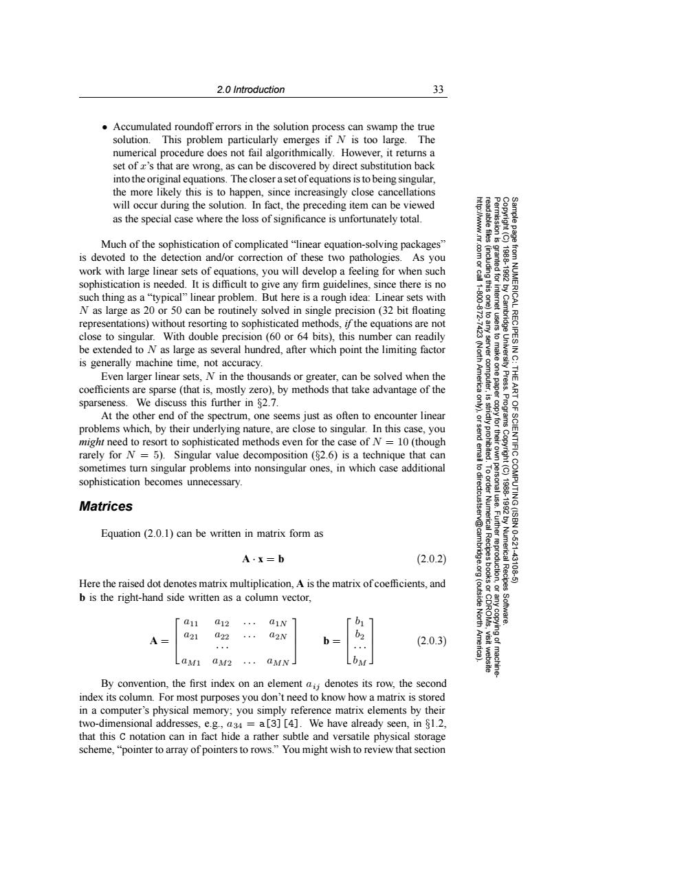
2.0 Introduction 33 Accumulated roundoff errors in the solution process can swamp the true solution.This problem particularly emerges if N is too large.The numerical procedure does not fail algorithmically.However,it returns a set of r's that are wrong,as can be discovered by direct substitution back into the original equations.The closer a set ofequations is to being singular the more likely this is to happen,since increasingly close cancellations will occur during the solution.In fact,the preceding item can be viewed as the special case where the loss of significance is unfortunately total. Much of the sophistication of complicated"linear equation-solving packages" is devoted to the detection and/or correction of these two pathologies.As you work with large linear sets of equations,you will develop a feeling for when such sophistication is needed.It is difficult to give any firm guidelines,since there is no such thing as a"typical"linear problem.But here is a rough idea:Linear sets with N as large as 20 or 50 can be routinely solved in single precision(32 bit floating representations)without resorting to sophisticated methods,if the equations are not close to singular.With double precision(60 or 64 bits),this number can readily RECIPES be extended to N as large as several hundred,after which point the limiting factor 会3川 is generally machine time,not accuracy. 9 Even larger linear sets,N in the thousands or greater,can be solved when the coefficients are sparse (that is,mostly zero),by methods that take advantage of the sparseness.We discuss this further in 82.7. At the other end of the spectrum,one seems just as often to encounter linear 9 problems which,by their underlying nature,are close to singular.In this case,you might need to resort to sophisticated methods even for the case of N=10(though rarely for N=5).Singular value decomposition($2.6)is a technique that can sometimes turn singular problems into nonsingular ones,in which case additional 61 sophistication becomes unnecessary. Matrices Equation(2.0.1)can be written in matrix form as Numerical Recipes 10.621 A·X=b (2.0.2) 43106 Here the raised dot denotes matrix multiplication,A is the matrix of coefficients,and b is the right-hand side written as a column vector, (outside Software. a11 012 aIN b1 North a21 A 022 a2N Y (2.0.3) A LaMi aM2 aMN bM By convention,the first index on an element ai;denotes its row,the second index its column.For most purposes you don't need to know how a matrix is stored in a computer's physical memory;you simply reference matrix elements by their two-dimensional addresses,e.g.,a34 =a[3][4].We have already seen,in $1.2. that this C notation can in fact hide a rather subtle and versatile physical storage scheme,"pointer to array of pointers to rows."You might wish to review that section2.0 Introduction 33 Permission is granted for internet users to make one paper copy for their own personal use. Further reproduction, or any copyin Copyright (C) 1988-1992 by Cambridge University Press. Programs Copyright (C) 1988-1992 by Numerical Recipes Software. Sample page from NUMERICAL RECIPES IN C: THE ART OF SCIENTIFIC COMPUTING (ISBN 0-521-43108-5) g of machine￾readable files (including this one) to any server computer, is strictly prohibited. To order Numerical Recipes books or CDROMs, visit website http://www.nr.com or call 1-800-872-7423 (North America only), or send email to directcustserv@cambridge.org (outside North America). • Accumulated roundoff errors in the solution process can swamp the true solution. This problem particularly emerges if N is too large. The numerical procedure does not fail algorithmically. However, it returns a set of x’s that are wrong, as can be discovered by direct substitution back into the original equations. The closer a set of equations is to being singular, the more likely this is to happen, since increasingly close cancellations will occur during the solution. In fact, the preceding item can be viewed as the special case where the loss of significance is unfortunately total. Much of the sophistication of complicated “linear equation-solving packages” is devoted to the detection and/or correction of these two pathologies. As you work with large linear sets of equations, you will develop a feeling for when such sophistication is needed. It is difficult to give any firm guidelines, since there is no such thing as a “typical” linear problem. But here is a rough idea: Linear sets with N as large as 20 or 50 can be routinely solved in single precision (32 bit floating representations) without resorting to sophisticated methods, if the equations are not close to singular. With double precision (60 or 64 bits), this number can readily be extended to N as large as several hundred, after which point the limiting factor is generally machine time, not accuracy. Even larger linear sets, N in the thousands or greater, can be solved when the coefficients are sparse (that is, mostly zero), by methods that take advantage of the sparseness. We discuss this further in §2.7. At the other end of the spectrum, one seems just as often to encounter linear problems which, by their underlying nature, are close to singular. In this case, you might need to resort to sophisticated methods even for the case of N = 10 (though rarely for N = 5). Singular value decomposition (§2.6) is a technique that can sometimes turn singular problems into nonsingular ones, in which case additional sophistication becomes unnecessary. Matrices Equation (2.0.1) can be written in matrix form as A · x = b (2.0.2) Here the raised dot denotes matrix multiplication, A is the matrix of coefficients, and b is the right-hand side written as a column vector, A =    a11 a12 ... a1N a21 a22 ... a2N ··· aM1 aM2 ... aMN    b =    b1 b2 ··· bM    (2.0.3) By convention, the first index on an element aij denotes its row, the second index its column. For most purposes you don’t need to know how a matrix is stored in a computer’s physical memory; you simply reference matrix elements by their two-dimensional addresses, e.g., a34 = a[3][4]. We have already seen, in §1.2, that this C notation can in fact hide a rather subtle and versatile physical storage scheme, “pointer to array of pointers to rows.” You might wish to review that section